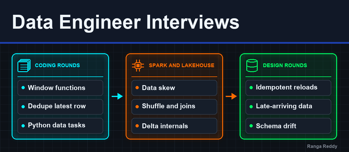
Top Data engineer interview questions
What 29 companies reportedly asked data engineers, merged into one list of unique questions, plus a component-wise bank for SQL, Python, Java, Scala, Spark, data modeling, system design, Airflow, Databricks, Snowflake and dbt. Every answer comes with full code and the output it produced.
- How the questions were collected
- How the answers were verified
- What each company focuses on
- What comes up most
- SQL
- Python and coding
- Spark architecture and execution
- Partitioning, shuffle and joins
- Data skew
- Memory and caching
- Performance and troubleshooting
- Streaming and Kafka
- Lakehouse and table formats
- Data modeling and warehousing
- Pipeline design and reliability
- Cloud services
- Behavioural and managerial rounds
- Interview questions by component
- How to prepare from this list
- References
- Trademarks
TL;DR
- Interview-experience posts from 29 companies, from Amazon and Netflix to the large IT services firms, collapse into 75 question groups once duplicates and near-duplicates are merged. Window functions came up at 19 of the 29; duplicates and idempotent reloads, slow-job investigations and late-arriving data at 12 or 13 each.
- Product companies (Amazon, Netflix, Atlassian, Grab, Paytm) spend their rounds on system design and failure scenarios. Services and consulting firms (TCS, Infosys, Cognizant, PwC, KPMG, Deloitte) spend theirs on Azure Data Factory, Databricks and SCD implementation, plus a managerial round.
- Treat company labels as hints, not facts. The same question list is posted under different company names, and some posts are verbatim copies across accounts. The questions are real interview material; which company asked a given question cannot be verified.
- A second, component-wise section adds 108 questions by skill: SQL, Python, Java, Scala, Spark, streaming, data modeling, system design, Airflow, Databricks, Snowflake, dbt, data quality, and LLM pipelines. Use it to drill one round at a time.
- Every technical answer has full code and the output it produced: the SQL ran on PostgreSQL, the PySpark on Spark with Delta Lake, Iceberg and Kafka, plus Python, Java, Scala, Airflow and dbt. Databricks, Snowflake and cloud-console code is marked as checked against the vendor’s documentation instead.
- Click a question to open its answer: the mechanism, the code, the trap, and the follow-up you should expect.
A list of “questions asked at company X” is only useful if it tells you what the interviewer is testing. Most of the posts these questions came from do not: they give a question title and move on, and the same thirty titles repeat under a different company name every week.
This post does the merging. It takes the questions from public LinkedIn interview-experience posts for data engineer roles, removes duplicates and near-duplicates, rewrites each one as a precise question, and groups them by the skill they test. Each technical question then gets an outline of what a strong answer covers, written the way the Spark interview questions post does it: the mechanism first, then the trap. Every answer that can run, did, and its output is printed under the code, so you can check your own version against it.
How the questions were collected
The source set is public LinkedIn posts from October 2026 that describe a data engineer interview at a named company, found through LinkedIn content search for “data engineer interview experience” and “interview experience PySpark SQL round”. Only posts that listed concrete questions were kept. Posts that described a process without questions, and posts for other roles (UX designer, GenAI engineer), were dropped.
Three things about this source are worth knowing before you use it:
The company attribution is weak. One twelve-question banking list appears word for word under Wipro, American Express and Databricks. One American Express post appears from four different accounts, one PayPal post from three, and one Cognizant post from three. Many of the posting accounts sell interview kits. Read a company label as “this question set circulated with this name on it”, not as a transcript.
The questions are still representative. The same question reaching you from five accounts says nothing about one company, but it says a lot about the market. The frequency counts below are the most reliable signal in the set.
Compensation figures were left out. The posts quote CTC ranges, but none can be checked, and they are not what you prepare against.
 public posts ──► keep posts that list questions ──► normalise wording
                                                        │
             ┌──────────────────────────────────────────┘
             ▼
   merge duplicates and near-duplicates ──► tag each question with
             │                              the companies it came from
             ▼
   group by skill ──► outline what a strong answer covers
How the answers were verified
Interview answers that only describe code are hard to check. Every answer here that could run was run, and the text under each code block is the output it produced:
- SQL: PostgreSQL 16.4, against the sample tables below. Spark SQL variants ran on Spark.
- PySpark: Spark 3.5.9 in
local[4]mode, with Delta Lake 3.3.2 and Apache Iceberg 1.11.0 tables on the local file system. - Streaming: Spark Structured Streaming reading from a Kafka broker, with throwaway topics deleted afterwards.
- Python: Python 3.10. Java: Java 17, as a single source file. Scala:
spark-shell(Scala 2.12). - Airflow: DAGs loaded with
DagBagand test-run withairflow dags teston Airflow 3.1.0. - dbt: dbt-core 1.10 with the DuckDB adapter.
Databricks-only features (Lakeflow pipelines, Unity Catalog, Auto Loader, system tables), Snowflake, and the Azure, GCP and AWS consoles cannot run locally. That code was checked against each vendor’s documentation, and each of those answers says so.
Running the code also corrected several first drafts, and those corrections
are in the answers: a late Kafka event that a watermark did not drop
(question 40), a runtime bloom filter that a boolean filter did not trigger
(question 28), a saveAsTable overwrite that open-source Delta rejects
(question 66), and two dbt rules the parser enforces (question
175).
The sample tables every SQL answer uses (PostgreSQL)
The data is small on purpose, and each table carries the edge case its questions are about: tied salaries, a missing month, two transactions at the same timestamp, a customer with no orders in February.
-- Sample data shared by every SQL answer in the post.
DROP TABLE IF EXISTS emp, logins, orders, txns, usage_monthly, accounts,
  account_audit, clicks, monthly_revenue, users, events, customer_raw,
  shipments, order_header, daily_sales, contacts, app_events, sellers,
  product_sales, visits, app_users, person, ride_users, trips, parcels,
  web_log, subscriptions, tasks, scores CASCADE;

CREATE TABLE emp (
  emp_id     int PRIMARY KEY,
  name       text NOT NULL,
  dept       text NOT NULL,
  salary     numeric(10,2) NOT NULL,
  manager_id int REFERENCES emp(emp_id),
  hire_date  date NOT NULL
);
INSERT INTO emp VALUES
  (1, 'Ranga',    'ENG',   250000, NULL, '2015-01-10'),
  (2, 'Nishanth', 'ENG',   180000, 1,    '2017-03-01'),
  (3, 'Meena',    'ENG',   180000, 1,    '2016-07-15'),
  (4, 'Vinod',    'ENG',   150000, 2,    '2019-11-20'),
  (5, 'Vasundra', 'SALES', 120000, 1,    '2018-02-01'),
  (6, 'Raja',     'SALES', 120000, 5,    '2020-05-05'),
  (7, 'Lakshmi',  'SALES', 95000,  5,    '2021-09-09'),
  (8, 'Kavi',     'HR',    90000,  1,    '2019-01-01'),
  (9, 'Manoj',    'ENG',   190000, 2,    '2022-04-04');   -- earns more than manager Nishanth

CREATE TABLE logins (user_id int, login_ts timestamp);
INSERT INTO logins VALUES
  (1,'2026-10-01 09:00'),(1,'2026-10-03 10:00'),(1,'2026-10-05 08:00'),
  (2,'2026-10-02 11:00'),
  (3,'2026-10-01 07:00'),(3,'2026-10-04 07:30');

CREATE TABLE orders (order_id int PRIMARY KEY, customer_id int, order_date date, amount numeric(10,2));
INSERT INTO orders VALUES
  (101, 1, '2026-01-05', 100), (102, 1, '2026-01-06', 50), (103, 1, '2026-01-07', 70),
  (104, 1, '2026-02-10', 40),
  (105, 2, '2026-01-15', 300),
  (106, 3, '2026-02-01', 80),  (107, 3, '2026-02-02', 20),
  (108, 4, '2026-01-20', 60),
  (109, 1, '2026-01-07', 10),  -- second order on the same day as 103
  (110, 1, '2025-06-10', 200), (111, 1, '2025-08-10', 150), (112, 1, '2025-10-10', 100),
  (113, 2, '2025-07-01', 50);   -- 2025 history for the baseline in question 14

CREATE TABLE txns (txn_id int, account_id int, txn_ts timestamp, amount numeric(10,2));
INSERT INTO txns VALUES                  -- txn_id records arrival order
  (1, 10,'2026-10-01 09:00:00', 500), (2, 10,'2026-10-01 09:00:00', -200),
  (3, 10,'2026-10-02 10:00:00', -50), (4, 20,'2026-10-01 12:00:00', 1000);

CREATE TABLE usage_monthly (user_id int, month date, usage int);
INSERT INTO usage_monthly VALUES
  (1,'2026-01-01',10),(1,'2026-02-01',12),(1,'2026-03-01',15),(1,'2026-04-01',9),
  (2,'2026-01-01',30),(2,'2026-02-01',25),(2,'2026-03-01',40),(2,'2026-04-01',45);

CREATE TABLE accounts (account_id int PRIMARY KEY, holder text);
INSERT INTO accounts VALUES (1,'Lakshmi'),(2,'Kavi'),(3,'Yashu'),(4,'Anada');
CREATE TABLE account_audit (account_id int, status text, changed_at timestamp);
INSERT INTO account_audit VALUES
  (1,'ACTIVE','2026-01-01'),(1,'SUSPENDED','2026-03-01'),
  (2,'SUSPENDED','2026-01-01'),(2,'ACTIVE','2026-02-01'),
  (3,'CLOSED','2026-02-15');            -- account 4 has no audit rows

CREATE TABLE clicks (user_id int, event_ts timestamp);
INSERT INTO clicks VALUES
  (1,'2026-10-01 09:00'),(1,'2026-10-01 09:10'),(1,'2026-10-01 09:55'),
  (1,'2026-10-01 10:05'),(2,'2026-10-01 12:00'),(2,'2026-10-01 12:20'),
  (2,'2026-10-01 12:50');                -- exactly 30 minutes later: same session

CREATE TABLE monthly_revenue (month date, product_id int, revenue numeric(10,2));
INSERT INTO monthly_revenue VALUES
  ('2026-01-01',1,100),('2026-02-01',1,0),('2026-04-01',1,150),   -- no March row
  ('2026-01-01',2,40),('2026-02-01',2,60),('2026-03-01',2,90);

CREATE TABLE users (user_id int PRIMARY KEY, signup_ts timestamp);
INSERT INTO users VALUES (1,'2026-01-03'),(2,'2026-01-20'),(3,'2026-02-02'),(4,'2026-02-10');
CREATE TABLE events (user_id int, event_ts timestamp);
INSERT INTO events VALUES
  (1,'2026-01-04'),(1,'2026-02-11'),(1,'2026-03-01'),
  (2,'2026-01-21'),(3,'2026-02-03'),(3,'2026-03-05'),(4,'2026-04-01');

CREATE TABLE customer_raw (customer_id int, email text, city text, updated_at timestamp, ingest_id int);
INSERT INTO customer_raw VALUES
  (1,'ranga@x.com','Pune',  '2026-01-01',1),(1,'ranga@x.com','Pune',  '2026-01-01',1),  -- exact duplicate
  (1,'ranga@x.com','Mumbai','2026-02-01',2),                                       -- newer version
  (2,'meena@x.com','Delhi', '2026-01-05',1),
  (3,'vinod@x.com','Chennai','2026-01-07',1),(3,'vinod.k@x.com','Chennai','2026-01-07',2); -- same ts, tiebreak

CREATE TABLE order_header (order_id int PRIMARY KEY, order_amount numeric(10,2));
INSERT INTO order_header VALUES (1,100),(2,200),(3,50);
CREATE TABLE shipments (shipment_id int, order_id int, carrier text, shipped_at timestamp);
INSERT INTO shipments VALUES (1,1,'DHL','2026-10-01'),(2,1,'DHL','2026-10-02'),(3,2,'UPS','2026-10-01');

CREATE TABLE daily_sales (sale_date date, region text, amount numeric(10,2));
INSERT INTO daily_sales VALUES
  ('2026-10-01','N',100),('2026-10-02','N',120),('2026-10-04','N',80),  -- 10-03 missing
  ('2026-10-05','N',90),('2026-10-01','S',50),('2026-10-02','S',55);

CREATE TABLE contacts (customer_id int, email text, updated_at date);
INSERT INTO contacts VALUES
  (14,'yashu@x.com','2026-02-02'),(27,'yashu@x.com','2026-02-19'),(31,'yashu@x.com','2026-02-24'),
  (9,'anada@x.com','2026-02-11'),(18,'anada@x.com','2026-02-11'),   -- tie on updated_at
  (22,'raja@x.com','2026-02-07'),
  (40,NULL,'2026-02-15'),(41,NULL,'2026-02-16');                     -- missing emails are never duplicates

CREATE TABLE app_events (user_id int, event_type text, event_ts timestamp);
INSERT INTO app_events VALUES
  (1,'login','2026-10-01 09:00'),(1,'view','2026-10-01 09:05'),(1,'view','2026-10-01 09:07'),
  (1,'add_to_cart','2026-10-01 09:10'),(1,'purchase','2026-10-01 09:15'),
  (2,'login','2026-10-02 10:00'),(2,'view','2026-10-02 10:02'),(2,'view','2026-10-02 10:04'),
  (2,'add_to_cart','2026-10-02 10:06'),
  (3,'login','2026-10-03 11:00'),(3,'purchase','2026-10-03 11:01'),   -- bought without a cart step
  (4,'login','2026-10-04 12:00');
CREATE TABLE app_users (user_id int PRIMARY KEY, signup_date date);
INSERT INTO app_users VALUES (1,'2026-09-28'),(2,'2026-09-29'),(3,'2026-09-30'),
                             (4,'2026-10-01'),(5,'2026-10-02');      -- user 5 never came back

CREATE TABLE sellers (seller_id int, signup_date date);
INSERT INTO sellers VALUES
  (1,'2021-04-11'),(2,'2021-09-30'),
  (3,'2022-01-05'),(4,'2022-03-17'),(5,'2022-06-21'),(6,'2022-08-02'),(7,'2022-12-12'),
  (8,'2024-02-14'),(9,'2024-05-01'),(10,'2024-07-19');                -- no sellers joined in 2023

CREATE TABLE product_sales (region text, product text, revenue numeric(10,2));
INSERT INTO product_sales VALUES
  ('East','Router',700),('East','Router',300),('East','Switch',450),
  ('East','Cable',450),('East','Adapter',120),('East','Mouse',30),
  ('West','Laptop',1200),('West','Monitor',650),('West','Dock',400);

CREATE TABLE visits (visit_date date, amount numeric(10,2));
INSERT INTO visits VALUES
  ('2026-10-01',40),('2026-10-02',55),('2026-10-03',65),('2026-10-04',80),
  ('2026-10-06',75),                                                  -- 5 October: the shop was closed
  ('2026-10-07',110),('2026-10-08',90),('2026-10-08',15),('2026-10-09',70);

CREATE TABLE person (id int PRIMARY KEY, email text);
INSERT INTO person VALUES
  (11,'kavi@x.com'),(12,'manoj@x.com'),(15,'kavi@x.com'),(19,'nishanth@x.com'),
  (23,'manoj@x.com'),(30,'Kavi@x.com');                  -- differs only in case

CREATE TABLE ride_users (user_id int PRIMARY KEY, banned text, role text);
INSERT INTO ride_users VALUES
  (21,'No','client'),(22,'Yes','client'),(23,'No','client'),(24,'No','client'),
  (31,'No','driver'),(32,'Yes','driver'),(33,'No','driver');   -- driver 34 is not in the table
CREATE TABLE trips (id int, client_id int, driver_id int, status text, request_date date);
INSERT INTO trips VALUES
  (1,21,31,'completed','2026-10-05'),(2,22,31,'cancelled_by_client','2026-10-05'),
  (3,23,33,'cancelled_by_driver','2026-10-05'),(4,21,33,'completed','2026-10-05'),
  (5,24,32,'cancelled_by_driver','2026-10-06'),(6,23,33,'completed','2026-10-06'),
  (7,24,34,'cancelled_by_client','2026-10-07');

CREATE TABLE parcels (parcel_id int, shipped_on date);
INSERT INTO parcels VALUES
  (1,'2026-01-05'),(2,'2026-01-15'),(3,'2026-01-31'),(4,'2026-02-01'),
  (5,'2026-04-10'),(6,'2026-04-11');                    -- nothing shipped in March

CREATE TABLE web_log (user_id int, event_type text, event_time timestamp);
INSERT INTO web_log VALUES
  (1,'page_load','2026-10-01 08:00'),(1,'page_exit','2026-10-01 08:12'),
  (1,'page_load','2026-10-01 08:30'),(1,'page_exit','2026-10-01 08:48'),
  (1,'page_load','2026-10-02 19:00'),(1,'page_exit','2026-10-02 19:24'),
  (2,'page_load','2026-10-01 23:50'),(2,'page_exit','2026-10-02 00:10'),  -- crosses midnight
  (2,'page_load','2026-10-02 08:00'),(2,'page_exit','2026-10-02 08:30'),
  (3,'page_load','2026-10-01 12:00');                                     -- never exits

CREATE TABLE subscriptions (sub_id int, user_id int, start_date date, end_date date);
INSERT INTO subscriptions VALUES
  (1,101,'2026-01-12','2026-01-28'),    -- cancelled inside its first month
  (2,102,'2026-01-20',NULL),            -- still active
  (3,103,'2026-01-05','2026-03-03'),
  (4,104,'2026-01-25','2026-02-01'),    -- ends exactly on the month-1 boundary: retained
  (5,105,'2026-02-03',NULL),
  (6,106,'2026-02-14','2026-04-30');

CREATE TABLE tasks (task_id int, task_date date, status text);
INSERT INTO tasks VALUES
  (1,'2026-10-10','completed'),(2,'2026-10-11','completed'),(3,'2026-10-12','completed'),
  (4,'2026-10-12','completed'),                      -- second task on the same day
  (5,'2026-10-13','pending'),                        -- not completed: breaks the run
  (6,'2026-10-14','completed'),
  (7,'2026-10-16','completed'),(8,'2026-10-17','completed');

CREATE TABLE scores (id int, score int);
INSERT INTO scores VALUES (1,91),(2,85),(3,91),(4,64),(5,85),(6,70),(7,85);
What each company focuses on
The table summarises the reported rounds for each company and the question that best captures what it tests. Companies are grouped by type, because the type predicts the interview better than the name does.
Product and platform companies
| Company | Reported rounds | Focus | Signature question |
|---|---|---|---|
| Amazon | Online assessment, technical deep dive, system design, bar raiser | Scale, cost, idempotency, leadership principles | 50 billion small files in S3 and queries slowing daily: give a remediation plan with no downtime |
| Microsoft | Coding (Python, SQL), Spark, end-to-end system design | SQL depth (self-join, recursive CTE), schema drift, SCD | Handle schema drift in a batch pipeline without breaking downstream tables |
| Netflix | SQL and modeling, PySpark, system design, production scenarios | Event data at scale, Iceberg table management | One task takes 45 minutes while the rest finish in 3. Why? |
| Atlassian | DSA, SQL, data system design, behavioural | Algorithms plus streaming design | Merge overlapping intervals, then design a real-time analytics pipeline with exactly-once semantics |
| Grab | SQL, Spark internals, project deep dive, design | Ride-sharing data model, small files in streaming | Small-file build-up in a high-throughput Kafka-fed pipeline |
| Walmart | SQL, Spark, DSA, project discussion | Consecutive-day patterns, migration, reconciliation | Daily sales reports are wrong after a deployment. Investigate. |
| Comcast | SQL, Spark, streaming | Partitioning, event time, freshness | Find customers whose monthly usage rose three months in a row |
| Ford | Pipeline design, Spark, data quality | Vehicle and sensor data, SCD Type 2 | Process millions of real-time vehicle sensor events |
Fintech and banking
| Company | Reported rounds | Focus | Signature question |
|---|---|---|---|
| Goldman Sachs | Modeling and SQL, big data, platform design, production and leadership | Trade data, table formats, lineage | Delta Lake vs Hudi vs Iceberg for a financial data lake |
| American Express | SQL and Python, Spark, architecture, HR | Recursive SQL, Spark memory, cost vs SLA | Optimise Spark cluster cost while holding the SLA |
| PayPal | Intro, SQL and Python, coding, design, behavioural | Payment ETL, late data, warehouse design | Design an ETL pipeline for payment transactions |
| Paytm | Design-heavy | Exactly-once, Kafka, fraud | Achieve exactly-once processing for payment events |
| HDFC Bank | ADF, Spark tuning, Delta scenario, SQL | Incremental snapshot design | Distinct phone numbers over 90 or 180 days of daily snapshots without scanning them all |
Data and analytics vendors
| Company | Reported rounds | Focus | Signature question |
|---|---|---|---|
| Databricks | Delta Lake, streaming, governance | Delta internals, Unity Catalog, multi-tenancy | A multi-terabyte Delta table has slowed down. Optimise it. |
| IBM | Coding, SQL, project | Window functions, Spark, Kafka basics | Second-highest salary without a subquery |
| Tiger Analytics | SQL, design, behavioural | Fundamentals, late data | Handle late-arriving data in pipelines |
| HCA Healthcare | SQL and PySpark, GCP architecture, debugging | Medallion on GCP, Airflow | Upstream data has not arrived while the DAG is running. What happens? |
Consulting and IT services
| Company | Reported rounds | Focus | Signature question |
|---|---|---|---|
| PwC | SQL and Python, ADF and Databricks, managerial | ADF runtime, MERGE, modeling | Azure IR vs self-hosted IR |
| EY | Spark, ADF, SQL | Retries, incremental loads | A pipeline fails halfway. Retry without duplicating data. |
| KPMG | SQL and Python, ADF and Databricks, managerial | ETL fundamentals, PySpark operations | Join two large datasets that run out of memory |
| Deloitte | Technical, case study, managerial | Migration, GDPR, lineage | Migrate 500 TB of banking history from Oracle to Synapse with zero downtime |
| Wipro | Banking-domain design | Compliance reporting, CDC, audit | Inconsistent balances in a regulatory report. Investigate. |
| Infosys | Technical, ADF and Delta, managerial | End-to-end pipeline explanation | repartition() vs coalesce() vs repartitionByRange() |
| TCS | Technical, technical and managerial, HR | Reusable ETL, banking pipelines | Design a reusable ETL framework for 20 clients with different schemas |
| Cognizant | Technical, Azure, managerial, HR | Azure end to end, cost | Databricks cluster cost doubled this month. Where do you start? |
| HCLTech | Advanced Spark, Delta and Azure | AQE, Delta internals, IaC | Row-level deletes in Delta without rewriting the partition |
| Capgemini | Technical, client technical | GCP plus Databricks | Penultimate order for every customer |
| Coforge | SQL and Python, PySpark and Databricks, client design | SCD2 with MERGE, idempotency | An ADF pipeline loads twice after a retry. Make it idempotent. |
| EPAM | Technical | ADF, Spark joins, Unity Catalog | Incremental load with no primary key and no timestamp |
What comes up most
Counting how many of the 29 companies each topic appeared under gives the clearest picture of where to spend preparation time. The counts come from the company tags on the questions below, so they are lower bounds: a post that only named a topic (“Spark optimisation”) without a question is not counted.
| Topic | Companies | Typical form |
|---|---|---|
| Window functions (rank, running totals, latest row) | 19 | Write it, then explain the tie behaviour |
| Duplicates and idempotent reloads | 13 | “The job ran twice” or “the source resent records” |
| Slow job investigation | 13 | “It used to take 2 hours, now 8” |
| Late-arriving data | 12 | Already-aggregated tables, reports |
| Data skew and salting | 10 | Diagnose from the Spark UI, then fix |
| SCD Type 2 | 10 | Implement with MERGE or in PySpark |
| Incremental load and CDC | 8 | Watermarks, MERGE |
| Delta Lake ACID and maintenance | 8 | Transaction log, OPTIMIZE, VACUUM |
| Schema evolution and drift | 6 | Without breaking downstream consumers |
repartition vs coalesce |
6 | Plus when each is wrong |
The pattern is clear: correctness under failure matters more than API recall. Duplicates, retries, late data and schema change make up most of the scenario questions, and they are all versions of one question: what happens to the data when something goes wrong.
SQL
Each question lists the companies it was reported under in brackets. Every query below runs against the sample tables in How the answers were verified, and the output under it is what PostgreSQL 16.4 returned.
Most SQL rounds reuse a small set of shapes. Recognising the shape is most of the work: the wording of the question tells you which one it is, and the shape tells you which window function or join to reach for. The SQL answers in this post fall into four families. Each answer names its pattern at the top, and covers the variants interviewers usually ask for.
Picking the right rows. Questions that say “top 3 per region”, “Nth
highest”, “latest record” or “remove duplicates” are ranking problems:
ROW_NUMBER(), RANK() or DENSE_RANK() over a partition, then a filter.
Top-N per group is in Q1, Q7 and Q10; deduplication in Q3.
Comparing a row with its neighbours. “Cumulative”, “rolling”, “compared with last month”, “in a row” and “idle for more than 30 minutes” all need a window that looks backwards:
- running totals, a
SUMwith aROWSframe: Q4; - moving averages, a frame of N rows or N days: Q85;
- period-over-period change,
LAGwithNULLIF: Q81; - gaps and islands, a date minus
ROW_NUMBER(): Q5; - sessions, a
LAGflag plus a runningSUM: Q76.
Following users over time. “Drop-off at each step” is a funnel, conditional counts per user (Q77). “Of the users who joined in March” is a retention cohort, a first month plus a month offset (Q80).
Reshaping and relating rows. “One column per month” is a pivot,
SUM(CASE ...) or FILTER (Q79). “Earns more than their manager”
is a self-join, the same table twice (Q83). “Everyone under this
manager” is a recursive CTE (Q8).
To practise, the SQL practice set later in this post works through eleven more problems that come up often in SQL screens.
The habit that pays off across all twelve: say out loud how the pattern breaks
on the edge cases before writing code. Ties, NULLs, missing dates, and a
second event on the same day account for most wrong answers.
1. Find the Nth highest salary, overall and per department, using more than one approach. [PwC, PayPal, Atlassian, IBM, Infosys, TCS, Capgemini, HCA Healthcare]
Pattern: top-N per group. The signal is “Nth highest” or “highest per”.
The sample emp table has a tie on purpose: Nishanth and Meena both earn
180,000 in ENG. A correct “second highest” must return the second distinct
salary, which is Manoj’s 190,000.
Approach 1, DENSE_RANK(). The default answer. Ties share a rank and no
rank is skipped, so rank 2 is the second distinct value.
-- 2nd highest distinct salary per department
SELECT dept, name, salary
FROM (
  SELECT dept, name, salary,
         DENSE_RANK() OVER (PARTITION BY dept ORDER BY salary DESC) AS rnk
  FROM emp
) t
WHERE rnk = 2
ORDER BY dept, name;
 dept  |  name   |  salary
-------+---------+-----------
 ENG   | Manoj   | 190000.00
 SALES | Lakshmi |  95000.00
(2 rows)
Approach 2, correlated subquery. For engines or interviewers that rule out window functions. A salary is the Nth highest when exactly N-1 distinct salaries in its department are greater. It re-scans the department for every row, so it is quadratic per group. Say that out loud.
-- Same answer without window functions (correlated subquery)
SELECT e1.dept, e1.name, e1.salary
FROM emp e1
WHERE 1 = (SELECT COUNT(DISTINCT e2.salary)
           FROM emp e2
           WHERE e2.dept = e1.dept AND e2.salary > e1.salary)
ORDER BY e1.dept, e1.name;
 dept  |  name   |  salary
-------+---------+-----------
 ENG   | Manoj   | 190000.00
 SALES | Lakshmi |  95000.00
(2 rows)
Approach 3, LIMIT ... OFFSET. Fine for the overall Nth value, awkward
per department. DISTINCT is what makes ties count once.
-- Overall Nth (N = 3) highest distinct salary
SELECT DISTINCT salary
FROM emp
ORDER BY salary DESC
LIMIT 1 OFFSET 2;
  salary
-----------
 180000.00
(1 row)
Approach 4, self-join with no ranking at all. The TCS and IBM variant
(“without RANK, LIMIT or a subquery”). The highest salary has nothing greater
than it, so it never appears on the left side of the join, and MAX of what
remains is the second highest.
-- Second highest overall without RANK, LIMIT or a subquery per row
SELECT MAX(e1.salary) AS second_highest
FROM emp e1
JOIN emp e2 ON e2.salary > e1.salary;
 second_highest
----------------
      190000.00
(1 row)
The trap: ROW_NUMBER() = 2 returns Nishanth or Meena, whichever the engine
happens to put second, and never Manoj. It answers “second row”, not “second
highest salary”.
2. ROW_NUMBER vs RANK vs DENSE_RANK, and when can a ROW_NUMBER solution be rewritten with DENSE_RANK? [PwC, EY, Walmart, Atlassian, Capgemini, IBM]
Run all three over the same ordering and the difference is visible on the tie:
SELECT dept, name, salary,
       ROW_NUMBER() OVER w AS row_number,
       RANK()       OVER w AS rank,
       DENSE_RANK() OVER w AS dense_rank
FROM emp
WHERE dept = 'ENG'
WINDOW w AS (ORDER BY salary DESC)
ORDER BY salary DESC, name;
 dept |   name   |  salary   | row_number | rank | dense_rank
------+----------+-----------+------------+------+------------
 ENG  | Ranga    | 250000.00 |          1 |    1 |          1
 ENG  | Manoj    | 190000.00 |          2 |    2 |          2
 ENG  | Meena    | 180000.00 |          4 |    3 |          3
 ENG  | Nishanth | 180000.00 |          3 |    3 |          3
 ENG  | Vinod    | 150000.00 |          5 |    5 |          4
(5 rows)
ROW_NUMBER()numbers rows 1, 2, 3, 4, 5 with no ties. Use it when you need exactly one row per group: deduplication, latest record.RANK()gives ties the same rank and then skips: 1, 2, 3, 3, 5. Competition ranking.DENSE_RANK()gives ties the same rank with no gap: 1, 2, 3, 3, 4. “Nth distinct value”.
They agree only when the ORDER BY key is unique within the partition. Once
there are ties, DENSE_RANK() = 1 returns several rows per group where
ROW_NUMBER() = 1 returns one, so a dedup query rewritten with DENSE_RANK
silently keeps duplicates.
Two common versions. “Rank scores without gaps” asks for each
distinct score with a gap-free rank, which is DENSE_RANK over DISTINCT
values:
-- Rank distinct scores with no gaps
SELECT score, DENSE_RANK() OVER (ORDER BY score DESC) AS rank
FROM (SELECT DISTINCT score FROM scores) s
ORDER BY score DESC;
 score | rank
-------+------
    91 |    1
    85 |    2
    70 |    3
    64 |    4
(4 rows)
Its RANK vs ROW_NUMBER
problem wants all three side by side, with ROW_NUMBER ties broken by name, which
makes the numbering deterministic:
-- All three ranks, with ROW_NUMBER ties broken by name
SELECT name, salary,
       RANK()       OVER (ORDER BY salary DESC)       AS rank_val,
       DENSE_RANK() OVER (ORDER BY salary DESC)       AS dense_rank_val,
       ROW_NUMBER() OVER (ORDER BY salary DESC, name) AS row_num
FROM emp
WHERE dept IN ('ENG', 'SALES')
ORDER BY salary DESC, name;
   name   |  salary   | rank_val | dense_rank_val | row_num
----------+-----------+----------+----------------+---------
 Ranga    | 250000.00 |        1 |              1 |       1
 Manoj    | 190000.00 |        2 |              2 |       2
 Meena    | 180000.00 |        3 |              3 |       3
 Nishanth | 180000.00 |        3 |              3 |       4
 Vinod    | 150000.00 |        5 |              4 |       5
 Raja     | 120000.00 |        6 |              5 |       6
 Vasundra | 120000.00 |        6 |              5 |       7
 Lakshmi  |  95000.00 |        8 |              6 |       8
(8 rows)
Meena and Nishanth tie on salary, so RANK gives both 3 and skips to 5,
DENSE_RANK gives both 3 and continues at 4, and ROW_NUMBER orders them by
name.
The follow-up is determinism. Look at the output: Nishanth got row number 3
and Meena 4, although they sort equal. That order is arbitrary. In Spark it
can change between runs, because partitions arrive in a different order.
Always add a tiebreaker column, such as ORDER BY salary DESC, emp_id.
3. Find duplicate records, delete them, and keep only the latest record per business key. [PwC, EY, Microsoft, PayPal, Tiger Analytics, Ford, HCA Healthcare]
Pattern: deduplication. The signal is “latest record”, “remove” or
“flag” duplicates. The core is always ROW_NUMBER() over the key, newest
first; what changes is whether you keep, delete or flag the other rows.
customer_raw holds three kinds of duplicate: an exact copy (customer 1
loaded twice), a newer version of the same key (customer 1 moved to Mumbai),
and two versions with the same timestamp (customer 3), which need a
tiebreaker.
Find them:
SELECT customer_id, COUNT(*) AS copies
FROM customer_raw
GROUP BY customer_id
HAVING COUNT(*) > 1
ORDER BY customer_id;
 customer_id | copies
-------------+--------
           1 |      3
           3 |      2
(2 rows)
Keep the latest, without changing the table. ingest_id breaks the tie
for customer 3:
SELECT customer_id, email, city, updated_at
FROM (
  SELECT *,
         ROW_NUMBER() OVER (PARTITION BY customer_id
                            ORDER BY updated_at DESC, ingest_id DESC) AS rn
  FROM customer_raw
) t
WHERE rn = 1
ORDER BY customer_id;
 customer_id |     email     |  city   |     updated_at
-------------+---------------+---------+---------------------
           1 | ranga@x.com   | Mumbai  | 2026-02-01 00:00:00
           2 | meena@x.com   | Delhi   | 2026-01-05 00:00:00
           3 | vinod.k@x.com | Chennai | 2026-01-07 00:00:00
(3 rows)
Delete in place. The table has no primary key, so there is nothing to tell
two identical rows apart. PostgreSQL’s physical row id, ctid, does that. SQL
Server uses a deletable CTE (WITH d AS (... ROW_NUMBER() ...) DELETE FROM d
WHERE rn > 1) for the same effect.
-- PostgreSQL: delete in place using the physical row id (ctid),
-- because the table has no primary key to tell the copies apart
DELETE FROM customer_raw c
USING (
  SELECT ctid,
         ROW_NUMBER() OVER (PARTITION BY customer_id
                            ORDER BY updated_at DESC, ingest_id DESC) AS rn
  FROM customer_raw
) d
WHERE c.ctid = d.ctid AND d.rn > 1;
SELECT customer_id, email, city FROM customer_raw ORDER BY customer_id;
 customer_id |     email     |  city
-------------+---------------+---------
           1 | ranga@x.com   | Mumbai
           2 | meena@x.com   | Delhi
           3 | vinod.k@x.com | Chennai
(3 rows)
In Delta, Iceberg or Hudi, do not delete row by row. Rewrite the affected
partitions with the deduplicated result (INSERT OVERWRITE, or MERGE from a
deduplicated source), so the change is one atomic commit.
Flag instead of delete. A common variant keeps every row and adds an
is_duplicate column. Two rules make it harder
than it looks: a missing email is never a duplicate, and a tie on
updated_at goes to the smallest ID.
-- Flag duplicates instead of deleting them: the newest row per email is kept
-- (ties go to the smallest customer_id), and a missing email is never a duplicate.
SELECT customer_id, email, updated_at,
       CASE WHEN email IS NULL THEN 0
            WHEN ROW_NUMBER() OVER (PARTITION BY email
                                    ORDER BY updated_at DESC, customer_id) = 1 THEN 0
            ELSE 1 END AS is_duplicate
FROM contacts
ORDER BY customer_id;
 customer_id |    email    | updated_at | is_duplicate
-------------+-------------+------------+--------------
           9 | anada@x.com | 2026-02-11 |            0
          14 | yashu@x.com | 2026-02-02 |            1
          18 | anada@x.com | 2026-02-11 |            1
          22 | raja@x.com  | 2026-02-07 |            0
          27 | yashu@x.com | 2026-02-19 |            1
          31 | yashu@x.com | 2026-02-24 |            0
          40 |             | 2026-02-15 |            0
          41 |             | 2026-02-16 |            0
(8 rows)
Without the email IS NULL branch, PARTITION BY email puts both NULL
emails into one group and flags customer 40, because SQL groups NULLs
together even though NULL = NULL is not true. Customers 9 and 18 share a date,
and the customer_id tiebreaker keeps 9.
The follow-up: an exact duplicate and a key duplicate are different
problems. The first is a DISTINCT. The second needs a rule for which version
wins, and that rule belongs to the business, not to you.
4. Running totals: claim amount per policy, account balance per transaction, sales per day. [Coforge, Wipro, American Express, Databricks, Microsoft, PayPal, Atlassian]
Pattern: running totals. The signal is “cumulative”, “balance” or “to date”.
Account 10 has two transactions at exactly the same timestamp. That is where the default window frame gives a wrong running balance.
The default frame is RANGE. With an ORDER BY and no frame clause, the
frame is RANGE BETWEEN UNBOUNDED PRECEDING AND CURRENT ROW. It includes every
peer row with the same txn_ts, so both 09:00 rows show the combined 300:
-- Default frame: RANGE, so rows with the same txn_ts are summed together
SELECT account_id, txn_ts, amount,
       SUM(amount) OVER (PARTITION BY account_id ORDER BY txn_ts) AS balance_range
FROM txns ORDER BY account_id, txn_ts, txn_id;
 account_id |       txn_ts        | amount  | balance_range
------------+---------------------+---------+---------------
         10 | 2026-10-01 09:00:00 |  500.00 |        300.00
         10 | 2026-10-01 09:00:00 | -200.00 |        300.00
         10 | 2026-10-02 10:00:00 |  -50.00 |        250.00
         20 | 2026-10-01 12:00:00 | 1000.00 |       1000.00
(4 rows)
State the frame as ROWS, and add a tiebreaker. Now each row shows the
balance after that transaction. The tiebreaker is txn_id, which records
arrival order:
-- Explicit ROWS frame, with arrival order (txn_id) breaking the timestamp tie
SELECT account_id, txn_id, txn_ts, amount,
       SUM(amount) OVER (PARTITION BY account_id
                         ORDER BY txn_ts, txn_id
                         ROWS BETWEEN UNBOUNDED PRECEDING AND CURRENT ROW) AS balance
FROM txns ORDER BY account_id, txn_ts, txn_id;
 account_id | txn_id |       txn_ts        | amount  | balance
------------+--------+---------------------+---------+---------
         10 |      1 | 2026-10-01 09:00:00 |  500.00 |  500.00
         10 |      2 | 2026-10-01 09:00:00 | -200.00 |  300.00
         10 |      3 | 2026-10-02 10:00:00 |  -50.00 |  250.00
         20 |      4 | 2026-10-01 12:00:00 | 1000.00 | 1000.00
(4 rows)
The same in PySpark:
from pyspark.sql import Window, functions as F

w = (Window.partitionBy("account_id")
           .orderBy("txn_ts", F.desc("amount"))
           .rowsBetween(Window.unboundedPreceding, Window.currentRow))
txns.withColumn("balance", F.sum("amount").over(w))
“In input order” needs a column. Interview versions of this pattern often
say “when several rows share a day, add them in their input order”. A SQL
table has no input order: without an ORDER BY on a real
column, the database may return rows in any order. Ask for, or create, a
column that records it: an ingestion sequence, a Kafka offset, or an
auto-increment ID.
For a balance, debits must already be negative. Say that you would check the
sign convention in the source, because a feed that stores debits as positive
numbers with a type column needs a CASE first.
5. Consecutive patterns: orders on consecutive days, usage rising three months in a row, a value appearing three times in a row. [Walmart, Comcast, American Express]
Pattern: gaps and islands. The signal is “consecutive”, “streak” or “in a row”. The classic version, “login streaks of three or more days”, is the same query as below with logins instead of orders.
LAG/LEAD for a fixed run length. “Rising three months in a row” means this month beats the last, and the last beat the one before:
-- Users whose usage rose three months in a row
SELECT user_id, month, usage
FROM (
  SELECT user_id, month, usage,
         LAG(usage, 1) OVER (PARTITION BY user_id ORDER BY month) AS prev1,
         LAG(usage, 2) OVER (PARTITION BY user_id ORDER BY month) AS prev2
  FROM usage_monthly
) t
WHERE usage > prev1 AND prev1 > prev2
ORDER BY user_id, month;
 user_id |   month    | usage
---------+------------+-------
       1 | 2026-03-01 |    15
       2 | 2026-04-01 |    45
(2 rows)
Gaps and islands for any run length. Subtract a row number from the date. Within a run of consecutive days the difference is constant, so it labels the run (the “island”):
-- Customers who ordered on 3 or more consecutive days (gaps and islands)
WITH days AS (
  SELECT DISTINCT customer_id, order_date FROM orders     -- one row per day first
),
grp AS (
  SELECT customer_id, order_date,
         order_date - (ROW_NUMBER() OVER (PARTITION BY customer_id
                                          ORDER BY order_date))::int AS island
  FROM days
)
SELECT customer_id, MIN(order_date) AS run_start, MAX(order_date) AS run_end,
       COUNT(*) AS days
FROM grp
GROUP BY customer_id, island
HAVING COUNT(*) >= 3;
 customer_id | run_start  |  run_end   | days
-------------+------------+------------+------
           1 | 2026-01-05 | 2026-01-07 |    3
(1 row)
Customer 1 has two orders on 7 January. The SELECT DISTINCT in the first CTE
matters: without it, the second order on the same day gets its own row number,
the subtraction shifts, and the run splits in two.
LAG needs one comparison per step, so it suits “exactly three”. Gaps and islands works for “three or more” and returns the run boundaries too.
Numbered date ranges. The “contiguous date ranges” variant adds two rules: only completed tasks count, and each run gets a sequential ID and an inclusive length. The status filter goes before the row numbering, so a pending day breaks the run:
-- Consecutive completed dates become one numbered interval
WITH done AS (
  SELECT DISTINCT task_date FROM tasks WHERE status = 'completed'
),
grp AS (
  SELECT task_date,
         task_date - (ROW_NUMBER() OVER (ORDER BY task_date))::int AS island
  FROM done
)
SELECT ROW_NUMBER() OVER (ORDER BY MIN(task_date)) AS project_id,
       MIN(task_date) AS start_date, MAX(task_date) AS end_date,
       MAX(task_date) - MIN(task_date) + 1 AS duration_days
FROM grp
GROUP BY island
ORDER BY start_date;
 project_id | start_date |  end_date  | duration_days
------------+------------+------------+---------------
          1 | 2026-10-10 | 2026-10-12 |             3
          2 | 2026-10-14 | 2026-10-14 |             1
          3 | 2026-10-16 | 2026-10-17 |             2
(3 rows)
12 October has two completed tasks and counts once, because of the DISTINCT.
13 October is pending, so the run from the 10th ends on the 12th. The duration
is end - start + 1, since both endpoints count.
When the source is timestamps, cast to a date first
(CAST(login_ts AS date)) and then deduplicate, so two logins on one day count
once. In Spark the subtraction is date_sub(login_date, rn); in Snowflake,
DATEADD(day, -rn, login_date).
6. Anti-joins: customers who ordered in January but not February at 100M rows, customers with no transaction in 90 days, LEFT SEMI vs LEFT ANTI, and missing records without a LEFT JOIN. [Cognizant, Wipro, American Express, EPAM]
NOT IN is the trap. One NULL in the subquery makes x NOT IN (...)
unknown for every row, and the query returns nothing:
-- NOT IN with a NULL in the subquery returns nothing
SELECT COUNT(*) AS rows_returned
FROM (VALUES (1), (2), (3)) c(id)
WHERE id NOT IN (SELECT x FROM (VALUES (1), (NULL)) s(x));
 rows_returned
---------------
             0
(1 row)
NOT EXISTS is the correct shape and is null-safe:
-- Customers who ordered in January but not in February
SELECT DISTINCT o.customer_id
FROM orders o
WHERE o.order_date >= '2026-01-01' AND o.order_date < '2026-02-01'
  AND NOT EXISTS (
    SELECT 1 FROM orders f
    WHERE f.customer_id = o.customer_id
      AND f.order_date >= '2026-02-01' AND f.order_date < '2026-03-01')
ORDER BY 1;
 customer_id
-------------
           2
           4
(2 rows)
Without any join, EXCEPT gives the same answer, at the cost of
deduplicating both sides:
SELECT customer_id FROM orders WHERE order_date >= '2026-01-01' AND order_date < '2026-02-01'
EXCEPT
SELECT customer_id FROM orders WHERE order_date >= '2026-02-01' AND order_date < '2026-03-01'
ORDER BY 1;
 customer_id
-------------
           2
           4
(2 rows)
In Spark, left_semi returns left rows that have a match, with no
right-hand columns and no duplication when the right side matches several
times. left_anti returns left rows with no match:
from pyspark.sql import functions as F

jan = orders.filter(F.col("order_date").between("2026-01-01", "2026-01-31"))
feb_customers = (orders
    .filter(F.col("order_date").between("2026-02-01", "2026-02-28"))
    .select("customer_id").distinct())          # shrink the right side first

jan.join(feb_customers, "customer_id", "left_anti").select("customer_id").distinct()
At 100M rows, both sides shuffle on customer_id. Reduce the right side to
distinct keys before the join, and keep the table partitioned by month so
each side is a single-partition scan. If the February key set is small enough,
F.broadcast(feb_customers) removes the shuffle of the large side entirely.
7. Second most recent login for every user, or the penultimate order for every customer. [PwC, Capgemini]
ROW_NUMBER() ... = 2 alone drops users with only one login. The interviewer
will ask about them, so answer it first: left join back to the distinct users.
-- Penultimate login per user, keeping users who have only one
WITH ranked AS (
  SELECT user_id, login_ts,
         ROW_NUMBER() OVER (PARTITION BY user_id ORDER BY login_ts DESC) AS rn
  FROM logins
)
SELECT u.user_id, r.login_ts AS second_latest_login
FROM (SELECT DISTINCT user_id FROM logins) u
LEFT JOIN ranked r ON r.user_id = u.user_id AND r.rn = 2
ORDER BY u.user_id;
 user_id | second_latest_login
---------+---------------------
       1 | 2026-10-03 10:00:00
       2 |
       3 | 2026-10-01 07:00:00
(3 rows)
User 2 has one login, so their second-latest login is NULL rather than
missing. If two logins share a timestamp, add a tiebreaker to the ORDER BY,
for the reason given in question 2.
8. Traverse a hierarchy (employees to managers, components to leaf parts) with a recursive CTE. [Microsoft, American Express]
Pattern: recursive hierarchies. The signal is “all reports under”, “chain of command” or “levels”.
The anchor member selects the root. The recursive member joins children to
the rows found so far. The path array does two jobs: it shows the chain, and
it is the cycle guard.
WITH RECURSIVE chain AS (
  SELECT emp_id, name, manager_id, 1 AS depth, ARRAY[emp_id] AS path
  FROM emp WHERE manager_id IS NULL
  UNION ALL
  SELECT e.emp_id, e.name, e.manager_id, c.depth + 1, c.path || e.emp_id
  FROM emp e
  JOIN chain c ON e.manager_id = c.emp_id
  WHERE NOT e.emp_id = ANY(c.path)      -- cycle guard
    AND c.depth < 20                    -- depth cap
)
SELECT emp_id, name, depth, path FROM chain ORDER BY path;
 emp_id |   name   | depth |  path
--------+----------+-------+---------
      1 | Ranga    |     1 | {1}
      2 | Nishanth |     2 | {1,2}
      4 | Vinod    |     3 | {1,2,4}
      9 | Manoj    |     3 | {1,2,9}
      3 | Meena    |     2 | {1,3}
      5 | Vasundra |     2 | {1,5}
      6 | Raja     |     3 | {1,5,6}
      7 | Lakshmi  |     3 | {1,5,7}
      8 | Kavi     |     2 | {1,8}
(9 rows)
Everyone under a given manager. The common variant starts the recursion at the manager’s direct reports instead of at the root, which also keeps the manager out of the result:
-- Everyone under a given manager, directly or indirectly, excluding the manager
WITH RECURSIVE reports AS (
  SELECT emp_id, name, manager_id, 1 AS level
  FROM emp WHERE manager_id = 2                       -- start at Nishanth's direct reports
  UNION ALL
  SELECT e.emp_id, e.name, e.manager_id, r.level + 1
  FROM emp e JOIN reports r ON e.manager_id = r.emp_id
)
SELECT emp_id, name, level FROM reports ORDER BY level, emp_id;
 emp_id | name  | level
--------+-------+-------
      4 | Vinod |     1
      9 | Manoj |     1
(2 rows)
Nishanth’s direct reports are Vinod and Manoj, and neither manages anyone, so the
recursion stops after one level. Starting the anchor at emp_id = 2 instead
would include Nishanth himself, which the question usually excludes.
Leaf nodes, the ones nobody reports to, are an anti-join on manager_id:
-- Leaf employees: nobody reports to them
SELECT e.emp_id, e.name
FROM emp e
WHERE NOT EXISTS (SELECT 1 FROM emp r WHERE r.manager_id = e.emp_id)
ORDER BY e.emp_id;
 emp_id |  name
--------+---------
      3 | Meena
      4 | Vinod
      6 | Raja
      7 | Lakshmi
      8 | Kavi
      9 | Manoj
(6 rows)
Name the two failure modes. A cycle in the data (A manages B, B manages A)
recurses forever, which is what the path check and the depth cap stop. And
the cost grows with depth, because every level is another join.
Spark 3.5 has no WITH RECURSIVE. The usual answer is a loop in the
driver that joins one level at a time and stops when a level comes back empty:
from pyspark.sql import functions as F

level = (emp.filter(F.col("manager_id").isNull())
            .select("emp_id", "name", F.lit(1).alias("depth")))
result = level
for depth in range(2, 21):                       # depth cap guards against cycles
    level = (emp.alias("e")
             .join(level.alias("l"), F.col("e.manager_id") == F.col("l.emp_id"))
             .select("e.emp_id", "e.name", F.lit(depth).alias("depth")))
    if level.isEmpty():                          # no new rows: the tree is done
        break
    result = result.unionByName(level)
+------+--------+-----+
|emp_id|    name|depth|
+------+--------+-----+
|     1|   Ranga|    1|
|     2|Nishanth|    2|
|     3|   Meena|    2|
|     5|Vasundra|    2|
|     4|   Vinod|    3|
|     6|    Raja|    3|
|     9|   Manoj|    3|
+------+--------+-----+
Each iteration adds a join to the plan, so for deep trees localCheckpoint()
the result every few levels to keep the lineage short.
9. List currently active accounts from an accounts table and a status-audit table, where accounts with no audit record count as active. [HDFC Bank]
Take the latest audit row per account, left join it to accounts, and treat a missing status as active:
WITH latest AS (
  SELECT account_id, status,
         ROW_NUMBER() OVER (PARTITION BY account_id ORDER BY changed_at DESC) AS rn
  FROM account_audit
)
SELECT a.account_id, COALESCE(l.status, 'ACTIVE') AS current_status
FROM accounts a
LEFT JOIN latest l ON l.account_id = a.account_id AND l.rn = 1
WHERE COALESCE(l.status, 'ACTIVE') = 'ACTIVE'
ORDER BY a.account_id;
 account_id | current_status
------------+----------------
          2 | ACTIVE
          4 | ACTIVE
(2 rows)
Account 1’s latest status is SUSPENDED, account 3’s is CLOSED, account 2 was reactivated, and account 4 has no audit rows at all. Account 4 is the point of the question: an inner join to the audit table drops it, and the “count as active” clause is how the interviewer checks whether you noticed.
10. Top 3 salaries per department, or top 3 products per region. [KPMG, Microsoft, Infosys]
Pattern: top-N per group. The signal is “top 3 per”, “highest in each”.
Ask first whether ties should all be returned. With DENSE_RANK(), ENG
returns four people for “top 3”, because two share third place:
SELECT dept, name, salary, rnk
FROM (
  SELECT dept, name, salary,
         DENSE_RANK() OVER (PARTITION BY dept ORDER BY salary DESC) AS rnk
  FROM emp
) t
WHERE rnk <= 3
ORDER BY dept, rnk, name;
 dept  |   name   |  salary   | rnk
-------+----------+-----------+-----
 ENG   | Ranga    | 250000.00 |   1
 ENG   | Manoj    | 190000.00 |   2
 ENG   | Meena    | 180000.00 |   3
 ENG   | Nishanth | 180000.00 |   3
 HR    | Kavi     |  90000.00 |   1
 SALES | Raja     | 120000.00 |   1
 SALES | Vasundra | 120000.00 |   1
 SALES | Lakshmi  |  95000.00 |   2
(8 rows)
Aggregate first, then rank. In the usual version the table holds
individual sales, so the ranking is over totals, not rows. Rank in
a second step, never in the same SELECT as the GROUP BY unless you mean to:
-- Aggregate first, then rank: top 3 revenue levels per region
WITH totals AS (
  SELECT region, product, SUM(revenue) AS total_revenue
  FROM product_sales GROUP BY region, product
),
ranked AS (
  SELECT *, DENSE_RANK() OVER (PARTITION BY region ORDER BY total_revenue DESC) AS region_rank
  FROM totals
)
SELECT region, product, total_revenue, region_rank
FROM ranked
WHERE region_rank <= 3
ORDER BY region, region_rank, product;
 region | product | total_revenue | region_rank
--------+---------+---------------+-------------
 East   | Router  |       1000.00 |           1
 East   | Cable   |        450.00 |           2
 East   | Switch  |        450.00 |           2
 East   | Adapter |        120.00 |           3
 West   | Laptop  |       1200.00 |           1
 West   | Monitor |        650.00 |           2
 West   | Dock    |        400.00 |           3
(7 rows)
Router’s two sales total 1,000. Cable and Switch tie at 450 and share rank 2, so East returns four products for “top 3”, and Mouse (30) is fourth by revenue level. Ranking before aggregating would rank the two Router rows separately, as 700 and 300.
If the requirement is “exactly three rows”, use ROW_NUMBER() with a
tiebreaker. In PySpark both are one window:
from pyspark.sql import Window, functions as F

w = Window.partitionBy("region").orderBy(F.desc("sales"))
(sales.withColumn("dense_rank", F.dense_rank().over(w))
      .withColumn("row_number", F.row_number().over(w.orderBy(F.desc("sales"), "product")))
      .filter("dense_rank <= 2"))
+------+-------+-----+----------+----------+
|region|product|sales|dense_rank|row_number|
+------+-------+-----+----------+----------+
|     N|     p1|  500|         1|         1|
|     N|     p2|  400|         2|         2|
|     N|     p3|  400|         2|         3|
|     S|     p1|  300|         1|         1|
|     S|     p5|  200|         2|         2|
+------+-------+-----+----------+----------+
11. A query that ran in 2 minutes now takes 20, or a query over billions of rows with several large joins needs optimising. [EY, Walmart, Comcast, PwC, KPMG, PayPal, EPAM, Ford]
Work from evidence, in this order:
- Compare the plans. Get the plan now and, if you can, from when it was fast. A changed join strategy, a lost index, or a filter that stopped pruning partitions explains most regressions.
- Check what changed. Data volume, stale statistics (which lead to bad join orders), a new predicate, or a function wrapped around a filter column.
- Reduce the bytes read. Partition and cluster on filter columns, select only the needed columns, push filters below joins.
- Fix the joins. Pre-aggregate before joining, filter early, broadcast the small side, and check for row explosion from many-to-many keys (question 82 shows one).
Reading a plan in PostgreSQL:
EXPLAIN (COSTS OFF)
SELECT o.customer_id, SUM(o.amount)
FROM orders o
WHERE o.order_date >= DATE '2026-01-01'
GROUP BY o.customer_id;
                     QUERY PLAN
----------------------------------------------------
 HashAggregate
   Group Key: customer_id
   ->  Seq Scan on orders o
         Filter: (order_date >= '2026-01-01'::date)
(4 rows)
A Seq Scan with a Filter on a large table is the first thing to question.
Use EXPLAIN (ANALYZE, BUFFERS) to get actual row counts and pages read, and
compare estimated rows with actual rows: a large gap means stale statistics,
so run ANALYZE orders.
The same check in Spark:
df.explain("formatted")       # physical plan, with PushedFilters on each scan
spark.sql("ANALYZE TABLE sales.orders COMPUTE STATISTICS FOR ALL COLUMNS")
The “it used to be fast” framing is deliberate. The interviewer wants to hear that you start with the plan diff, not with adding indexes.
12. NULL semantics: in aggregates, joins and filters, and what happens with a = null, b = null, a == b? [Comcast, PayPal, Tiger Analytics, KPMG]
One query shows most of it:
SELECT NULL = NULL                   AS eq,
       NULL IS NOT DISTINCT FROM NULL AS null_safe_eq,
       COUNT(*)                       AS count_star,
       COUNT(x)                       AS count_col,
       AVG(x)                         AS avg_col
FROM (VALUES (10), (NULL), (20)) t(x);
 eq | null_safe_eq | count_star | count_col |       avg_col
----+--------------+------------+-----------+---------------------
    | t            |          3 |         2 | 15.0000000000000000
(1 row)
- Comparison:
NULL = NULLisNULL(the blank ineq), not true, so aWHEREdrops the row. UseIS NULL,IS NOT DISTINCT FROM, Spark’s<=>, oreqNullSafein PySpark. - Aggregates:
COUNT(*)counts 3 rows,COUNT(x)counts 2, andAVG(x)is 15, not 10, because the null is skipped rather than treated as zero. - Grouping:
GROUP BYputs all nulls into one group.
Joins: null keys never match, even with each other:
SELECT COUNT(*) AS matched_rows
FROM (VALUES (NULL::int), (1)) a(k)
JOIN (VALUES (NULL::int), (1)) b(k) ON a.k = b.k;
 matched_rows
--------------
            1
(1 row)
In PySpark the null-safe version does match them:
a.join(b, a.k == b.k).count()             # 1
a.join(b, a.k.eqNullSafe(b.k)).count()    # 2
equi-join rows    : 1
null-safe join rows: 2
13. SQL fundamentals asked as quick checks: CTE vs subquery, GROUP BY vs HAVING, TRUNCATE vs DELETE, indexing, materialized views. [KPMG, Tiger Analytics, PayPal, Capgemini]
WHERE vs HAVING. WHERE filters rows before grouping, HAVING filters
groups after:
SELECT dept, COUNT(*) AS staff, AVG(salary)::int AS avg_salary
FROM emp
WHERE hire_date >= '2017-01-01'          -- filters rows before grouping
GROUP BY dept
HAVING COUNT(*) >= 2                     -- filters groups after
ORDER BY dept;
 dept  | staff | avg_salary
-------+-------+------------
 ENG   |     3 |     173333
 SALES |     3 |     111667
(2 rows)
CTE vs subquery. Most engines produce the same plan. A CTE is more
readable and can be referenced twice. PostgreSQL 12 and later inline a CTE
unless you write AS MATERIALIZED, so a CTE is not automatically computed
once.
TRUNCATE vs DELETE. DELETE FROM t WHERE ... removes chosen rows, fires
row triggers, and is fully logged. TRUNCATE t removes all rows by
deallocating storage, with no WHERE. In PostgreSQL both are transactional
and can be rolled back; in some other engines TRUNCATE cannot.
Index.
CREATE INDEX idx_orders_customer_date ON orders (customer_id, order_date);
A sorted structure that turns a scan into a seek. It costs write throughput
and storage, and a composite index helps a filter on its leading column, not
on order_date alone.
Materialized view.
CREATE MATERIALIZED VIEW daily_revenue AS
SELECT order_date, SUM(amount) AS revenue FROM orders GROUP BY order_date;

REFRESH MATERIALIZED VIEW daily_revenue;
A stored query result that trades freshness for read cost. On a lakehouse the “index” question becomes partitioning, clustering and file-level statistics, because Parquet tables have no B-tree indexes.
14. Find customers whose purchases in the last 90 days exceed their average monthly purchase by more than 50%. [Deloitte]
Define the baseline before writing SQL. Here it is the average month over the
six months before the 90-day window, counting months with no purchases as
zero. Then “exceeds by 50%” means the last 90 days are more than
1.5 × (3 × average month).
-- Customers whose last-90-day spend is more than 50% above their usual
-- 90-day spend, where "usual" is the average month over the 6 months before
-- the window, counting months with no purchases as zero.
WITH params AS (SELECT DATE '2026-02-28' AS as_of),
months AS (
  SELECT generate_series(DATE '2025-06-01', DATE '2025-11-01', INTERVAL '1 month')::date AS m
),
monthly AS (
  SELECT customer_id, DATE_TRUNC('month', order_date)::date AS m, SUM(amount) AS total
  FROM orders GROUP BY 1, 2
),
baseline AS (
  SELECT c.customer_id, AVG(COALESCE(mo.total, 0)) AS avg_month
  FROM (SELECT DISTINCT customer_id FROM orders) c
  CROSS JOIN months m
  LEFT JOIN monthly mo ON mo.customer_id = c.customer_id AND mo.m = m.m
  GROUP BY c.customer_id
),
recent AS (
  SELECT customer_id, SUM(amount) AS last_90d
  FROM orders, params
  WHERE order_date > as_of - 90 AND order_date <= as_of
  GROUP BY customer_id
)
SELECT r.customer_id, r.last_90d, ROUND(b.avg_month, 2) AS avg_month,
       ROUND(b.avg_month * 3 * 1.5, 2) AS threshold
FROM recent r JOIN baseline b USING (customer_id)
WHERE b.avg_month > 0                       -- no baseline: a new customer, not a spike
  AND r.last_90d > 1.5 * b.avg_month * 3
ORDER BY 1;
 customer_id | last_90d | avg_month | threshold
-------------+----------+-----------+-----------
           2 |   300.00 |      8.33 |     37.50
(1 row)
Customer 2 spent 50 in the baseline (8.33 a month) and 300 in the last 90 days, so it is flagged. Customer 1 averaged 75 a month, giving a threshold of 337.50, and spent 270, so it is not.
The trap is the zero months. Months with no rows do not exist in a
GROUP BY, so averaging only the months that have orders overstates the
baseline. Customer 1 ordered in three of the six baseline months. Without the
calendar CTE its average would be 150, not 75. Generate a month calendar and
LEFT JOIN to it, as above.
Also decide what to do with customers who have no baseline at all. This query
excludes them (avg_month > 0), because a new customer is not a spike.
Python and coding
These rounds are about clean, correct code under pressure, not about algorithms rarely seen in data engineering. Every snippet ran on Python 3.10, and the output under it is from that run.
15. Data-shaped Python: deduplicate a list keeping order, count frequencies, find duplicate employees by ID, group consecutive numbers into ranges. [PwC, EY, Azure-role interviews]
from collections import Counter, defaultdict

def dedupe_keep_order(items):
    return list(dict.fromkeys(items))          # dicts keep insertion order

def duplicates_by_key(records, key):
    groups = defaultdict(list)
    for r in records:
        groups[r[key]].append(r)
    return {k: v for k, v in groups.items() if len(v) > 1}

def consecutive_ranges(nums):
    out = []
    for x in sorted(set(nums)):
        if out and x == out[-1][1] + 1:
            out[-1][1] = x                     # extend the current range
        else:
            out.append([x, x])                 # start a new one
    return [f"{a}-{b}" if a != b else str(a) for a, b in out]

print(dedupe_keep_order([3, 1, 3, 2, 1]))
print(Counter("mississippi").most_common(2))
emps = [{"id": 1, "name": "A"}, {"id": 2, "name": "B"}, {"id": 1, "name": "A2"}]
print(duplicates_by_key(emps, "id"))
print(consecutive_ranges([1, 2, 3, 7, 8, 10]))
[3, 1, 2]
[('i', 4), ('s', 4)]
{1: [{'id': 1, 'name': 'A'}, {'id': 1, 'name': 'A2'}]}
['1-3', '7-8', '10']
Give the complexity for each. All are O(n), except the ranges, which are
O(n log n) because of the sort. most_common returns ties in the order the
elements were first seen, so i comes before s here.
16. Classic algorithm questions: merge overlapping intervals, longest substring without repeating characters, longest consecutive sequence, first non-repeating character, pairs summing to a target, top K frequent elements. [Atlassian, PwC, Walmart, PayPal, Tiger Analytics]
import heapq
from collections import Counter, OrderedDict

def merge_intervals(iv):                       # O(n log n)
    out = []
    for s, e in sorted(iv):
        if out and s <= out[-1][1]:
            out[-1][1] = max(out[-1][1], e)
        else:
            out.append([s, e])
    return out

def longest_unique_substring(s):               # O(n) sliding window
    last, start, best = {}, 0, 0
    for i, ch in enumerate(s):
        if ch in last and last[ch] >= start:
            start = last[ch] + 1
        last[ch] = i
        best = max(best, i - start + 1)
    return best

def longest_consecutive(nums):                 # O(n)
    s, best = set(nums), 0
    for x in s:
        if x - 1 not in s:                     # only start counting at a run's start
            n = 1
            while x + n in s:
                n += 1
            best = max(best, n)
    return best

def first_non_repeating(s):                    # O(n)
    c = Counter(s)
    return next((ch for ch in s if c[ch] == 1), None)

def pairs_with_sum(nums, target):              # O(n)
    seen, pairs = set(), set()
    for x in nums:
        if target - x in seen:
            pairs.add((min(x, target - x), max(x, target - x)))
        seen.add(x)
    return sorted(pairs)

def top_k_frequent(items, k):                  # O(n log k)
    return [x for x, _ in heapq.nlargest(k, Counter(items).items(), key=lambda kv: kv[1])]

class FirstUnique:
    """First non-repeating element of a stream, O(1) per event."""
    def __init__(self):
        self.candidates = OrderedDict()
        self.repeated = set()
    def add(self, x):
        if x in self.repeated:
            return
        if x in self.candidates:
            del self.candidates[x]
            self.repeated.add(x)
        else:
            self.candidates[x] = None
    def first(self):
        return next(iter(self.candidates), None)

print(merge_intervals([[1, 3], [2, 6], [8, 10], [9, 12]]))
print(longest_unique_substring("abcabcbb"))
print(longest_consecutive([100, 4, 200, 1, 3, 2]))
print(first_non_repeating("swiss"))
print(pairs_with_sum([2, 7, 4, 5, 3, 6], 9))
print(top_k_frequent(["a", "b", "a", "c", "b", "a"], 2))
fu = FirstUnique()
for x in [5, 3, 5, 7, 3]:
    fu.add(x)
print("first unique in stream:", fu.first())
[[1, 6], [8, 12]]
3
4
w
[(2, 7), (3, 6), (4, 5)]
['a', 'b']
first unique in stream: 7
For “first non-repeating element in a stream” (PayPal), the follow-up is
memory. FirstUnique keeps only the current candidates in order plus a set of
values already seen twice, so each event is O(1) and the stream itself is never
stored.
17. Flatten nested JSON, process a multi-GB CSV without loading it into memory, and compute top routes by revenue without pandas. [Coforge, Microsoft, Tiger Analytics, PwC, KPMG]
Flatten nested JSON. Recursion over dicts and lists, joining keys with a separator:
def flatten(obj, parent="", sep="."):
    out = {}
    if isinstance(obj, dict):
        for k, v in obj.items():
            out.update(flatten(v, f"{parent}{sep}{k}" if parent else k, sep))
    elif isinstance(obj, list):
        for i, v in enumerate(obj):
            out.update(flatten(v, f"{parent}{sep}{i}" if parent else str(i), sep))
    else:
        out[parent] = obj
    return out

order = {"id": 7, "customer": {"name": "Ranga", "address": {"city": "Pune"}},
         "items": [{"sku": "A", "qty": 2}, {"sku": "B", "qty": 1}]}
print(flatten(order))

def explode_items(order):
    """The other choice for lists: one output row per list element."""
    base = {k: v for k, v in flatten(order).items() if not k.startswith("items.")}
    return [{**base, **{f"item.{k}": v for k, v in item.items()}} for item in order["items"]]

for row in explode_items(order):
    print(row)
{'id': 7, 'customer.name': 'Ranga', 'customer.address.city': 'Pune', 'items.0.sku': 'A', 'items.0.qty': 2, 'items.1.sku': 'B', 'items.1.qty': 1}
{'id': 7, 'customer.name': 'Ranga', 'customer.address.city': 'Pune', 'item.sku': 'A', 'item.qty': 2}
{'id': 7, 'customer.name': 'Ranga', 'customer.address.city': 'Pune', 'item.sku': 'B', 'item.qty': 1}
Ask which one the interviewer wants. Indexed keys keep one row per order; exploding gives one row per item. The row count changes, and so does every sum downstream.
Large CSV and top routes without pandas. Stream with csv.DictReader,
which holds one line at a time, and keep only the aggregate in memory. The
test file has 200,000 trips:
import csv, heapq
from collections import defaultdict

def top_routes(path, k=3):
    revenue = defaultdict(float)
    with open(path, newline="") as fh:          # one line in memory at a time
        for row in csv.DictReader(fh):
            revenue[(row["origin"], row["dest"])] += float(row["fare"])
    return heapq.nlargest(k, revenue.items(), key=lambda kv: kv[1])

for route, rev in top_routes(path):
    print(route, round(rev, 2))
('A', 'X') 348084.34
('B', 'W') 347387.78
('C', 'X') 345089.67
Memory is proportional to the number of distinct routes, not to the file. For anything that needs a sort or a join across the whole file, say you would hand it to DuckDB or Spark rather than write an external sort by hand.
18. Python language questions: decorators, multithreading vs multiprocessing, mutable vs immutable objects, exceptions. [American Express, Data QA interviews]
Decorator. A function that takes a function and returns a wrapped one. A retry decorator is the example worth giving, because it is what data engineers actually write:
import time
from functools import wraps

def retry(times=3, base_delay=0.01, exceptions=(Exception,)):
    def deco(fn):
        @wraps(fn)                             # keep fn's name and docstring
        def wrapper(*args, **kwargs):
            for attempt in range(1, times + 1):
                try:
                    return fn(*args, **kwargs)
                except exceptions:
                    if attempt == times:
                        raise                  # re-raise the last error unchanged
                    time.sleep(base_delay * 2 ** (attempt - 1))
        return wrapper
    return deco

calls = {"n": 0}

@retry(times=3, exceptions=(ConnectionError,))
def flaky():
    """Fails twice, then succeeds."""
    calls["n"] += 1
    if calls["n"] < 3:
        raise ConnectionError("transient")
    return "ok"

print(flaky(), "after", calls["n"], "calls; name kept:", flaky.__name__,
      "| doc kept:", flaky.__doc__)
ok after 3 calls; name kept: flaky | doc kept: Fails twice, then succeeds.
Retry only the exceptions that can succeed on retry. A ValueError from bad
data will fail the same way three times.
Threads vs processes. CPython’s GIL lets one thread run Python bytecode at a time, so threads help I/O-bound work (waiting on a network or disk releases the GIL) and processes help CPU-bound work:
from concurrent.futures import ThreadPoolExecutor

def io_task(_):
    time.sleep(0.2)                             # stands in for a network call
    return 1

t0 = time.perf_counter()
with ThreadPoolExecutor(8) as ex:
    list(ex.map(io_task, range(8)))
print(f"8 x 0.2s sleeps on 8 threads finished in under 0.5s: {time.perf_counter() - t0 < 0.5}")
8 x 0.2s sleeps on 8 threads finished in under 0.5s: True
For CPU-bound work, ProcessPoolExecutor has the same interface; question
99 uses it.
Mutability. Lists, dicts and sets are mutable; tuples, strings and frozensets are not. Question 93 shows the classic bug, a mutable default argument, and question 94 shows shallow versus deep copies.
Exceptions. Catch the narrowest exception you can handle, use finally or
a with block for cleanup, and re-raise with raise (not raise e) to keep
the original traceback.
Spark architecture and execution
Every PySpark snippet in the Spark sections ran on Spark 3.5.9 in local[4]
mode. Plan text is trimmed to the lines that matter, and the expression IDs
(#123L) will differ on your machine.
19. What happens, end to end, when a Spark application is submitted? [Grab, Azure-role interviews]
spark-submit \
  --master yarn --deploy-mode cluster \
  --num-executors 10 --executor-cores 4 --executor-memory 8g \
  --conf spark.sql.shuffle.partitions=400 \
  daily_orders.py --date 2026-10-01
spark-submitstarts the driver. Inclusterdeploy mode it runs inside the cluster (on YARN, in the ApplicationMaster container); inclientmode it runs on the machine you submitted from.- The driver creates the
SparkSessionand asks the cluster manager (YARN, Kubernetes or standalone) for executors. - Your code builds a logical plan. Nothing executes yet.
- An action (
count,collect,write) hands the plan to Catalyst, which analyses it, optimises it and picks a physical plan. - The DAG scheduler cuts the physical plan into stages at every shuffle boundary.
- The task scheduler sends one task per partition of each stage to executor cores.
- Map-side tasks write shuffle files to local disk; the next stage’s tasks fetch them over the network.
- Results go back to the driver (
collect) or are written to storage by the executors (write).
The follow-up is always “where does it break?”: the driver on collect() or a
large broadcast, executors at a shuffle or on a skewed partition, and the
cluster manager when it cannot grant the containers you asked for (the
application then sits in ACCEPTED on YARN, or pods stay Pending on
Kubernetes).
20. Given a sequence (read CSV, repartition(2), filter, select, groupBy, collect), say how many jobs, stages and tasks Spark creates. [Azure-role interviews]
Do not guess: ask Spark. The status tracker reports every job and stage a job group created. The CSV here is written as 4 files.
from pyspark.sql import functions as F

def count_work(group, fn):
    sc.setJobGroup(group, group)
    fn()
    jobs = sc.statusTracker().getJobIdsForGroup(group)
    stages = []
    for j in sorted(jobs):
        for s in sc.statusTracker().getJobInfo(j).stageIds:
            info = sc.statusTracker().getStageInfo(s)
            if info is not None:
                stages.append((j, s, info.numTasks))
    return sorted(jobs), stages

def pipeline():
    df = spark.read.option("header", True).option("inferSchema", True).csv(csv_path)
    (df.repartition(2)
       .filter(F.col("amount") > 10)
       .select("customer_id", "amount")
       .groupBy("customer_id").agg(F.sum("amount"))
       .collect())

jobs, stages = count_work("seq", pipeline)                    # AQE on (the default)
spark.conf.set("spark.sql.adaptive.enabled", "false")
jobs, stages = count_work("seq_noaqe", pipeline)              # AQE off
jobs: 5
  job 0  stage 56  tasks 1
  job 1  stage 57  tasks 4
  job 2  stage 58  tasks 4
  job 3  stage 60  tasks 2
  job 3  stage 59  tasks 4
  job 4  stage 63  tasks 1
  job 4  stage 61  tasks 4
  job 4  stage 62  tasks 2
with AQE disabled, jobs: 3
  job 0  stage 64  tasks 1
  job 1  stage 65  tasks 4
  job 2  stage 66  tasks 4
  job 2  stage 67  tasks 2
  job 2  stage 68  tasks 200
Read it with AQE off first, because that is the textbook answer:
- Job 0, 1 task: reading the header. With
header=true, Spark reads the first line to get the column names. - Job 1, 4 tasks:
inferSchema. A full pass over all 4 files to work out the types. This is the job the question is designed to catch. - Job 2, the
collect(), 3 stages: the scan (4 tasks, one per file split), the stage afterrepartition(2)(2 tasks), and the stage after thegroupByshuffle (spark.sql.shuffle.partitions, 200 tasks).
With AQE on, the job count rises to 5. AQE runs each shuffle stage as its own job so it can look at the real sizes before planning the next one, and it coalesced the final 200 partitions into 1. Both answers are correct for their settings. Say which one you are describing.
Passing an explicit schema removes jobs 0 and 1 entirely, which is also the answer to “how would you make this faster”.
21. Narrow vs wide transformations, transformations vs actions, and lazy evaluation. [Capgemini, Azure-role interviews, HCA Healthcare]
A narrow transformation (filter, select, withColumn) computes each
output partition from one input partition. A wide one (groupBy, join,
distinct, repartition) needs rows from many partitions, so it forces a
shuffle, and the shuffle is a stage boundary. In the plan, the shuffle is the
Exchange node:
df = spark.range(0, 1000).withColumn("k", F.col("id") % 10)
df.filter("id > 5").select("k").groupBy("k").count().explain()
== Physical Plan ==
AdaptiveSparkPlan isFinalPlan=false
+- HashAggregate(keys=[k#257L], functions=[count(1)])
   +- Exchange hashpartitioning(k#257L, 200), ENSURE_REQUIREMENTS, [plan_id=2145]
      +- HashAggregate(keys=[k#257L], functions=[partial_count(1)])
         +- Project [(id#255L % 10) AS k#257L]
            +- Filter (id#255L > 5)
               +- Range (0, 1000, step=1, splits=4)
Everything below Exchange (range, filter, project, partial count) runs in one
stage without moving data. The Exchange hashpartitioning(k, 200) moves rows
so that each key lands in one partition. Note the two HashAggregate nodes:
Spark counts within each partition before the shuffle (partial_count), so
only 10 partial results per partition cross the network, not 1,000 rows.
Transformations vs actions. Transformations only add to the plan; actions
(collect, count, write, show) run it. Laziness is what lets Catalyst
see the whole query, push the filter down to the scan, and drop unused
columns before anything runs.
22. RDD vs DataFrame vs Dataset, and SparkContext vs SparkSession. [HCA Healthcare, American Express, Azure-role interviews]
from pyspark.sql import SparkSession

spark = SparkSession.builder.appName("orders").getOrCreate()   # the entry point
sc = spark.sparkContext                                         # the lower-level handle

# RDD: Python objects and lambdas. Spark cannot see inside them.
rdd = sc.parallelize([("A", 10), ("B", 5), ("A", 7)])
totals_rdd = rdd.reduceByKey(lambda a, b: a + b)

# DataFrame: named, typed columns. Catalyst can optimise this.
df = spark.createDataFrame(rdd, "customer STRING, amount INT")
totals_df = df.groupBy("customer").sum("amount")
An RDD is a distributed collection of objects with no schema. Spark cannot
reorder or prune what it cannot see, and in Python every row is serialized to a
Python worker. A DataFrame carries a schema, so Catalyst prunes columns
and pushes filters, and Tungsten stores rows in a compact binary format off
the Python heap. A Dataset (Scala and Java only) is a typed DataFrame,
Dataset[Order]; in Python only the DataFrame exists. Question
122 shows the one cost of the typed API.
SparkSession (since 2.0) is the single entry point for SQL, DataFrames and
the catalog. It wraps a SparkContext, the lower-level connection to the
cluster that RDDs and accumulators still use.
23. What is the Catalyst optimizer, and what is predicate pushdown? [Grab, Comcast, Azure-role interviews]
Catalyst turns a query into a parsed plan, resolves names against the catalog
(the analysed plan), applies rule-based rewrites such as predicate pushdown,
constant folding and column pruning (the optimised plan), then chooses a
physical plan. Whole-stage code generation compiles chains of operators into
one JVM function; the *(1) prefixes in a plan mark them.
Predicate pushdown moves a filter into the data source, so less data is read at all:
spark.read.parquet(pq).filter("customer_id = 7 AND amount > 500") \
     .select("order_id", "amount").explain()
== Physical Plan ==
*(1) Project [order_id#279L, amount#281]
+- *(1) Filter (((isnotnull(customer_id#280L) AND isnotnull(amount#281)) AND (customer_id#280L = 7)) AND (amount#281 > 500.0))
   +- *(1) ColumnarToRow
      +- FileScan parquet [order_id#279L,customer_id#280L,amount#281] Batched: true, DataFilters: [isnotnull(customer_id#280L), isnotnull(amount#281), (customer_id#280L = 7), (amount#281 > 500.0)], Format: Parquet, Location: InMemoryFileIndex(1 paths)[file:/tmp/qa_spark/orders_parquet], PartitionFilters: [], PushedFilters: [IsNotNull(customer_id), IsNotNull(amount), EqualTo(customer_id,7), GreaterThan(amount,500.0)], ReadSchema: struct<order_id:bigint,customer_id:bigint,amount:double>
Three things to point at in that scan node:
PushedFilters: the predicates handed to the Parquet reader, which uses row-group min/max statistics to skip row groups that cannot match.ReadSchema: only three columns are read, although the file may have more. That is column pruning.- The
Filterabove the scan stays. Pushdown skips row groups, not individual rows, so Spark still filters the rows it reads.
A JDBC source pushes the same filters into the database’s WHERE clause.
24. How does Spark decide the number of partitions, and what is a good target partition size? [Comcast, Azure-role interviews]
File scans split files into chunks of at most
spark.sql.files.maxPartitionBytes (128 MB by default), packing small files
together using spark.sql.files.openCostInBytes. One 337 MB Parquet file,
read twice:
for mb in (128, 32):
    spark.conf.set("spark.sql.files.maxPartitionBytes", f"{mb}m")
    print(f"maxPartitionBytes={mb}m -> partitions:", spark.read.parquet(big).rdd.getNumPartitions())
file size: 337 MB
maxPartitionBytes=128m -> partitions: 4
maxPartitionBytes=32m -> partitions: 11
shuffle partitions default: 200
Four partitions at 128 MB, not three. The split size also takes
spark.sql.files.minPartitionNum (the default parallelism, 4 here) into
account, so Spark makes splits smaller to keep every core busy. The file count
alone does not set the partition count.
Shuffles produce spark.sql.shuffle.partitions partitions (200), which
AQE then coalesces toward spark.sql.adaptive.advisoryPartitionSizeInBytes
(64 MB). Question 128 shows 200 becoming 1.
Explicitly, repartition(n) and coalesce(n) set it.
A useful target is 100 to 200 MB of input per task. Much smaller and scheduling overhead dominates; much larger and tasks spill and run long.
Partitioning, shuffle and joins
25. repartition() vs coalesce() vs repartitionByRange(): what happens internally and when to use each. [EY, Walmart, Infosys, American Express, HDFC Bank, TCS, Azure-role interviews]
Start from 8 equal partitions of 100,000 rows and look at the row counts per partition:
base = spark.range(0, 100_000, numPartitions=8)
sizes = lambda d: d.rdd.glom().map(len).collect()

print("original        :", sizes(base))
print("coalesce(3)     :", sizes(base.coalesce(3)))
print("repartition(3)  :", sizes(base.repartition(3)))
r = base.repartitionByRange(3, "id")
print("byRange(3)      :", sizes(r))
original        : [12500, 12500, 12500, 12500, 12500, 12500, 12500, 12500]
coalesce(3)     : [25000, 37500, 37500]
repartition(3)  : [33335, 33332, 33333]
byRange(3)      : [33498, 33080, 33422]
byRange min/max : [(0, 33497), (33498, 66577), (66578, 99999)]
coalesce(3)merges existing partitions without a shuffle, so the result is uneven (25,000 against 37,500). It can only reduce the partition count.repartition(3)does a full shuffle (round-robin, or hash when you pass columns), so the result is even. It can increase or decrease.repartitionByRange(3, "id")samples the column to choose boundaries, then shuffles, so each partition holds a contiguous, non-overlapping range. Use it before writing sorted output, so files have tight min/max statistics.
The trap: coalesce(1) before a write does not just produce one file.
With no shuffle to separate them, it pulls the whole upstream stage down to
one task, so the entire computation runs single-threaded. repartition(1)
keeps upstream parallelism and pays for one shuffle instead.
26. How does a broadcast join work, when do you avoid it, and what if neither side is small? [American Express, HCLTech, EPAM, Netflix, Azure-role interviews]
The driver collects the small side, builds a hash table, and ships it to every
executor, so the large side joins where it sits with no shuffle. Spark picks it
when a side’s estimated size is below spark.sql.autoBroadcastJoinThreshold
(10 MB):
facts = spark.range(0, 1_000_000).withColumn("cust", F.col("id") % 1000)
dim = spark.range(0, 1000).withColumnRenamed("id", "cust").withColumn("segment", F.lit("gold"))

facts.join(dim, "cust").explain()                    # automatic

spark.conf.set("spark.sql.autoBroadcastJoinThreshold", "-1")
facts.join(dim, "cust").explain()                    # broadcast disabled

facts.join(F.broadcast(dim), "cust").explain()       # hint overrides the threshold
== Physical Plan ==
AdaptiveSparkPlan isFinalPlan=false
+- Project [cust#313L, id#311L, gold AS segment#320]
   +- BroadcastHashJoin [cust#313L], [cust#318L], Inner, BuildRight, false
      :- Project [id#311L, (id#311L % 1000) AS cust#313L]
      :  +- Filter isnotnull((id#311L % 1000))
      :     +- Range (0, 1000000, step=1, splits=4)
      +- BroadcastExchange HashedRelationBroadcastMode(List(input[0, bigint, false]),false), [plan_id=2309]
         +- Project [id#316L AS cust#318L]
            +- Range (0, 1000, step=1, splits=4)


--- threshold -1, AQE off:
== Physical Plan ==
*(5) Project [cust#313L, id#311L, gold AS segment#320]
+- *(5) SortMergeJoin [cust#313L], [cust#318L], Inner
   :- *(2) Sort [cust#313L ASC NULLS FIRST], false, 0
   :  +- Exchange hashpartitioning(cust#313L, 200), ENSURE_REQUIREMENTS, [plan_id=2347]
   :     +- *(1) Project [id#311L, (id#311L % 1000) AS cust#313L]
   :        +- *(1) Filter isnotnull((id#311L % 1000))
   :           +- *(1) Range (0, 1000000, step=1, splits=4)
   +- *(4) Sort [cust#318L ASC NULLS FIRST], false, 0
      +- Exchange hashpartitioning(cust#318L, 200), ENSURE_REQUIREMENTS, [plan_id=2353]
         +- *(3) Project [id#316L AS cust#318L]
            +- *(3) Range (0, 1000, step=1, splits=4)


--- explicit hint:
== Physical Plan ==
*(2) Project [cust#313L, id#311L, gold AS segment#320]
+- *(2) BroadcastHashJoin [cust#313L], [cust#318L], Inner, BuildRight, false
   :- *(2) Project [id#311L, (id#311L % 1000) AS cust#313L]
   :  +- *(2) Filter isnotnull((id#311L % 1000))
   :     +- *(2) Range (0, 1000000, step=1, splits=4)
   +- BroadcastExchange HashedRelationBroadcastMode(List(input[0, bigint, false]),false), [plan_id=2406]
      +- *(1) Project [id#316L AS cust#318L]
         +- *(1) Range (0, 1000, step=1, splits=4)
With the threshold disabled, the same join becomes a SortMergeJoin with an
Exchange and a Sort on both sides: the million-row side is shuffled too.
The hint brings back BroadcastHashJoin regardless of the threshold.
Avoid it when the small side is big once decompressed into a hash table,
because it must fit in driver memory and in every executor. A forced hint on a
wrong size estimate is a common cause of driver OOM, and of
spark.sql.broadcastTimeout (300 seconds) failures.
When neither side is small: filter and project both sides first,
pre-aggregate if the join is followed by a groupBy, bucket both tables on the
join key for joins you run repeatedly (question 27), and let AQE switch to a
broadcast at runtime if a side turns out small after filtering.
27. Broadcasting vs bucketing, and partitioning vs bucketing. [KPMG, Azure-role interviews]
Partitioning splits a table into directories by column value, so queries skip whole directories. It suits low-cardinality filter columns such as date:
df.write.partitionBy("order_date").parquet("s3://lake/orders") # .../order_date=2026-10-01/
Bucketing hashes a column into a fixed number of files. Two tables bucketed the same way on the join key can join with no shuffle. It suits high-cardinality join keys:
spark.conf.set("spark.sql.autoBroadcastJoinThreshold", "-1")   # rule out broadcast

(orders.write.bucketBy(8, "cust").sortBy("cust").saveAsTable("orders_b"))
(customers.write.bucketBy(8, "cust").sortBy("cust").saveAsTable("customers_b"))

plan = spark.table("orders_b").join(spark.table("customers_b"), "cust") \
            ._jdf.queryExecution().executedPlan().toString()
print("Exchange in bucketed join plan:", "Exchange" in plan)
Exchange in bucketed join plan: False
Exchange when one side is not bucketed: True
Both tables bucketed on cust into 8 buckets: no Exchange. Join the
bucketed table to an unbucketed one and the shuffle comes back. Bucketing
needs saveAsTable, because the bucket spec lives in the catalog, and both
sides must use the same bucket count.
Broadcasting is a per-query choice for one small table. Bucketing is a layout paid once at write time, for large joins you run every day.
28. What are bloom filters, and how do they speed up joins? [American Express]
A bloom filter is a compact bit array that answers “definitely not present” or “possibly present”. Built from the join keys of the filtered small side, it lets the large side drop rows that cannot match before the shuffle.
Spark injects one at runtime when the creation side has a selective filter and the application side is large. The size threshold defaults to 10 GB, so the demo lowers it:
spark.conf.set("spark.sql.autoBroadcastJoinThreshold", "-1")
spark.conf.set("spark.sql.optimizer.runtime.bloomFilter.applicationSideScanSizeThreshold", "1KB")

fact = spark.read.parquet(f"{base}/fact_bloom")                     # 2M rows
vip = spark.read.parquet(f"{base}/dim_bloom").filter(F.col("tier") == "vip")
q = fact.join(vip, "cust")
plan = q._jdf.queryExecution().optimizedPlan().toString()
print("bloom filter injected:", "might_contain" in plan)
bloom filter injected: True
Filter (isnotnull(cust#17L) AND might_contain(scalar-subquery#31 [], xxhash64(cust#17L, 42)))
  +- Aggregate [bloom_filter_agg(xxhash64(cust#20L, 42), 1000000, 8388608, 0, 0) AS bloomFilter#30]
The bloom_filter_agg builds the filter from the VIP customers, and the
might_contain filter on the fact side drops non-matching rows during the
scan. It is controlled by spark.sql.optimizer.runtime.bloomFilter.enabled,
which is true by default since Spark 3.3.
A failed first attempt worth knowing: filtering the dimension on a bare
boolean column, .filter("vip"), injected nothing. Spark only builds a filter
when the creation side has a predicate it considers selective, such as an
equality, IN or LIKE.
Parquet and Delta also store bloom filters per column for point lookups on high-cardinality fields, where min/max statistics cannot prune.
29. Joining two large datasets runs out of memory. What do you do? [KPMG, Netflix, Azure-role interviews]
Find where it fails before changing anything:
- Driver OOM (
java.lang.OutOfMemoryErrorin the driver log, often duringBroadcastExchange): a broadcast that was too large. Remove the hint, or lower the threshold. - Executor OOM or a container killed for exceeding memory, on one or two tasks: skew. One key’s rows do not fit in one task. See question 30.
- Every task spilling heavily: too few shuffle partitions for the data size.
Then, in order:
# 1. Shrink both sides before the join
left = big_a.filter("event_date >= '2026-10-01'").select("cust", "amount")
right = big_b.select("cust", "segment").dropDuplicates(["cust"])   # check the key is unique

# 2. More, smaller shuffle partitions, so each task holds less
spark.conf.set("spark.sql.shuffle.partitions", "2000")
spark.conf.set("spark.sql.adaptive.enabled", "true")
spark.conf.set("spark.sql.adaptive.skewJoin.enabled", "true")

# 3. Check for row explosion before blaming memory
print(left.groupBy("cust").count().orderBy(F.desc("count")).first())
print(right.groupBy("cust").count().filter("count > 1").count())   # many-to-many?

joined = left.join(right, "cust")
A many-to-many key multiplies rows (10,000 × 10,000 matches on one key is 100 million output rows), and no memory setting fixes that. Raising executor memory is the last step, not the first.
Data skew
30. How do you identify data skew in the Spark UI? One task runs 45 minutes while the rest finish in 3. [Netflix, Comcast, Azure-role interviews]
In the Spark UI, open the slow stage and read the summary metrics table: compare Max with Median for Duration, Shuffle Read Size and Records. A max many times the median, on a stage right after a shuffle, is skew. Spill on that one task confirms it.
Then find the key. The test data puts 60% of a million events on
user_id = 0:
events = (spark.range(0, 1_000_000)
          .withColumn("user_id", F.when(F.col("id") % 10 < 6, F.lit(0))
                                   .otherwise(F.col("id") % 10_000)))

events.groupBy("user_id").count().orderBy(F.desc("count")).show(3)
print(events.repartition(8, "user_id").rdd.glom().map(len).collect())
+-------+------+
|user_id| count|
+-------+------+
|      0|600000|
|     26|   100|
|     29|   100|
+-------+------+
only showing top 3 rows

partition sizes after hash shuffle on user_id (8 partitions):
[49100, 50400, 49300, 52200, 49000, 650900, 48700, 50400]
After a hash shuffle into 8 partitions, one partition holds 650,900 rows and
the other seven about 50,000 each. That one partition is the 45-minute task.
In real data the hot key is usually a NULL, a default such as 0 or
'UNKNOWN', or one very large customer.
31. Fix skew: AQE skew join, salting, and what to do when AQE is disabled or one key holds 60% of the rows. [HCLTech, Coforge, American Express, HDFC Bank, PwC, Ford, HCA Healthcare]
Fix 1, AQE skew join. On by default since Spark 3.2. It splits a shuffle partition that is both 5 times the median and larger than 256 MB, and replicates the matching partition from the other side. These are the settings it uses:
spark.sql.adaptive.enabled = true
spark.sql.adaptive.skewJoin.enabled = true
spark.sql.adaptive.skewJoin.skewedPartitionFactor = 5.0
spark.sql.adaptive.skewJoin.skewedPartitionThresholdInBytes = 268435456b
spark.sql.adaptive.coalescePartitions.enabled = true
spark.sql.adaptive.advisoryPartitionSizeInBytes = 67108864b
It acts only on sort-merge and shuffled hash joins, and only above both
thresholds, so a 200 MB hot partition is left alone. Lower
skewedPartitionThresholdInBytes if your partitions are small.
Fix 2, salting. Spread the hot key across N sub-keys on the large side, and replicate the other side N times so every sub-key still finds its match:
N = 8
salted_events = events.withColumn("salt", (F.rand(7) * N).cast("int"))
salted_users = users.crossJoin(spark.range(N).withColumnRenamed("id", "salt"))
joined = salted_events.join(salted_users, ["user_id", "salt"]).drop("salt")

print("salted join rows:", joined.count(), " plain join rows:", events.join(users, "user_id").count())
print(salted_events.filter("user_id = 0").repartition(8, "user_id", "salt").rdd.glom().map(len).collect())
salted join rows: 1000000  plain join rows: 1000000
hot key spread over partitions after salting:
[74936, 225227, 149636, 0, 0, 75260, 0, 74941]
Same row count as the plain join, so the result is correct. The 600,000 hot rows now land in several partitions instead of one. Hash collisions put two salts in the same partition here, which is why salting with N = 8 does not give 8 equal pieces.
Choosing N (HDFC asked this directly): roughly the hot key’s size divided by the target partition size. A 6 GB hot key with a 256 MB target needs about 24. Too small leaves the partition hot; too large multiplies the other side by N for nothing.
Fix 3, when one key is 60% of the data. First ask whether that key should be joined at all. If it is a null or a placeholder, filter it out and union it back. If it is real, join it separately with a broadcast of its single matching row:
hot = events.filter("user_id = 0")
rest = events.filter("user_id <> 0")
out = (rest.join(users, "user_id")
       .unionByName(hot.join(F.broadcast(users.filter("user_id = 0")), "user_id")))
rows: 1000000
The hot rows never shuffle, because the other side of their join is one row.
Memory and caching
32. cache() vs persist(): default storage levels, what happens when cached data does not fit, and how to release it. [HCLTech, Cognizant, Azure-role interviews]
from pyspark import StorageLevel

c = spark.range(0, 1000)
c.cache()
print("DataFrame cache level:", c.storageLevel)
c.count()                                   # caching is lazy: this fills it
print("is_cached:", c.is_cached)
c.unpersist()

r = sc.parallelize(range(10)).cache()
print("RDD cache level      :", r.getStorageLevel())

p = spark.range(0, 10).persist(StorageLevel.DISK_ONLY)
print("persist(DISK_ONLY)   :", p.storageLevel)
DataFrame cache level: Disk Memory Deserialized 1x Replicated
is_cached: True
RDD cache level      : Memory Serialized 1x Replicated
persist(DISK_ONLY)   : Disk Serialized 1x Replicated
cache() is persist() with the default level, and the default differs: a
DataFrame uses memory and disk, an RDD memory only. persist(level) picks
another.
When it does not fit: with a memory-and-disk level, blocks that do not fit are written to local disk; with memory only, they are dropped and recomputed from lineage the next time they are needed. Cached data shares the unified memory pool with execution, so caching too much slows shuffles and sorts.
Release it with unpersist(), or spark.catalog.clearCache() for
everything. Cache only a DataFrame that is reused by more than one action, and
check the Storage tab for the fraction actually cached.
33. Spark memory management, driver vs executor memory, and why a job hits OOM despite enough cluster resources. [American Express, Netflix, Azure-role interviews]
Work the numbers for an 8 GB executor:
def executor_memory(heap_mb, memory_fraction=0.6, storage_fraction=0.5,
                    overhead_factor=0.10, reserved_mb=300):
    usable = heap_mb - reserved_mb
    unified = usable * memory_fraction            # execution + storage, shared
    return {
        "unified pool (execution + storage)": round(unified),
        "storage protected from eviction": round(unified * storage_fraction),
        "user memory (your objects, UDF state)": round(usable - unified),
        "overhead, off-heap (container extra)": round(max(384, heap_mb * overhead_factor)),
    }

for k, v in executor_memory(8192).items():
    print(f"{k:40s} {v:>6} MB")
unified pool (execution + storage)         4735 MB
storage protected from eviction            2368 MB
user memory (your objects, UDF state)      3157 MB
overhead, off-heap (container extra)        819 MB
The container asks the cluster manager for heap plus overhead, about 9 GB. Execution (shuffles, joins, sorts, aggregations) and storage (cache) share the unified pool; execution can evict cached blocks, but not below the protected storage share.
OOM with ample cluster capacity is a per-task problem, because one task’s data must fit in one executor:
- one skewed partition (question 30);
- an oversized broadcast, which fails in the driver;
collect()ortoPandas()on a large result, also the driver;- Python UDF workers or Arrow buffers outgrowing overhead, which shows up as
Container killed by YARN for exceeding memory limitsorOOMKilledon Kubernetes, not as a Java heap error. The fix there isspark.executor.memoryOverhead, not more heap.
Performance and troubleshooting
34. A job that took 2 hours now takes 8 (or 3x or 4x longer). Walk through the investigation. [Wipro, Deloitte, TCS, Databricks, EY, Azure-role interviews]
- What changed? Input volume, code, cluster, configs, upstream schema. Most regressions are a change nobody announced.
- Compare the Spark UI of a good run and a bad run stage by stage, and find the stage whose time grew. The history server keeps old runs.
- In that stage, check input size, shuffle size, spill, the task-time distribution (skew), GC time, and failed or retried tasks.
- Check the storage layer: small files accumulating, a filter that stopped pruning partitions, a table growing without compaction.
- Fix the cause and verify on comparable data.
Pull the stage metrics programmatically from the history server, so the comparison is numbers, not screenshots:
import requests

HS = "http://history-server:18080/api/v1"

def stage_summary(app_id):
    stages = requests.get(f"{HS}/applications/{app_id}/stages", timeout=30).json()
    return {s["name"][:60]: {"seconds": s["executorRunTime"] // 1000,
                             "input_mb": s["inputBytes"] // 2**20,
                             "shuffle_read_mb": s["shuffleReadBytes"] // 2**20,
                             "spill_mb": s["diskBytesSpilled"] // 2**20}
            for s in stages if s["status"] == "COMPLETE"}

good, bad = stage_summary("app-good"), stage_summary("app-bad")
for name in bad:
    if name in good and bad[name]["seconds"] > 2 * good[name]["seconds"]:
        print(name, good[name], "->", bad[name])
Interviewers listen for a hypothesis tested against evidence, not a list of tuning parameters.
35. A Spark job or streaming query gets slower over days or weeks. What do you look at? [Azure-role interviews, Netflix]
Look for the things that grow without bound:
- Small files in the input table. Each run lists and opens more files.
- Streaming state with no watermark. State is never dropped, so every batch reads and writes a larger state store.
stateOperators[].numRowsTotalin the query progress shows it growing. - Table metadata without maintenance. Delta logs without checkpoints, Iceberg snapshots never expired.
- A lookup table that used to be broadcast and has grown past the threshold, so the join silently became a sort-merge join.
Watch the trend from inside the job:
q = df.writeStream.option("checkpointLocation", chk).toTable("silver.events")
p = q.lastProgress
print(p["batchId"], p["durationMs"]["triggerExecution"],
      [s["numRowsTotal"] for s in p["stateOperators"]])
A triggerExecution that grows with numRowsTotal is unbounded state.
36. Too many small files: in a PySpark job, a streaming pipeline, or 50 billion files in an S3 lake. [Amazon, Comcast, Grab, HCLTech, Netflix]
Prevent them. Repartition by the table’s partition columns before writing, so each task writes to one partition directory instead of all of them:
(df.repartition("order_date")                  # one task per date
   .write.partitionBy("order_date").mode("append").parquet(path))
For streaming, use a longer trigger interval, so each micro-batch writes fewer, larger files.
Repair them with compaction. 20 appends of 5 files each made 100 small
files; OPTIMIZE rewrote them as one:
spark.sql(f"OPTIMIZE delta.`{s}` ZORDER BY (cust)") \
     .select("metrics.numFilesAdded", "metrics.numFilesRemoved").show()
files before: 100
+-------------+---------------+
|numFilesAdded|numFilesRemoved|
+-------------+---------------+
|            1|            100|
+-------------+---------------+

files after: 1
The equivalents are CALL catalog.system.rewrite_data_files('db.tbl') in
Iceberg and clustering in Hudi. The table format commits the rewrite
atomically, so readers see either the old files or the new ones, never a mix.
That is how you compact with no downtime. The old files stay until VACUUM
(or snapshot expiry) removes them.
At 50 billion files, listing itself is the bottleneck. A table format replaces directory listing with a metadata scan, and compaction then runs in batches, partition by partition, starting with the partitions queried most.
37. How do you size a cluster for 100 GB, optimise a 500 GB CSV, or cut Spark cost while holding the SLA? [Azure-role interviews, TCS, American Express, Cognizant]
Size from partitions, then cores:
input_gb, target_mb = 100, 128
tasks = input_gb * 1024 // target_mb               # 800 tasks
cores_per_executor, executors = 5, 20
waves = tasks / (cores_per_executor * executors)   # 8 waves of 100 tasks
print(tasks, waves)
Eight waves of 100 concurrent tasks is reasonable. Then check the shuffle
volume in a test run, which is often larger than the input, and size
spark.sql.shuffle.partitions from it.
A 500 GB CSV:
schema = "order_id BIGINT, customer_id BIGINT, amount DECIMAL(12,2), order_ts TIMESTAMP"
df = (spark.read.schema(schema)                 # no inference pass over 500 GB
      .option("header", True).csv("s3://landing/orders/*.csv"))
(df.withColumn("order_date", F.to_date("order_ts"))
   .write.partitionBy("order_date").parquet("s3://lake/orders"))  # convert once
An explicit schema removes the inference pass (question 20 shows it is a full extra job). Make sure the file is splittable: one 500 GB gzip file is read by a single task. Convert to Parquet once if it will be read again.
Cut cost while holding the SLA: autoscaling with a sensible maximum, spot or preemptible workers for stateless stages, compaction so fewer tasks run, removing caches nobody reuses, and measuring cost per run before and after each change.
Streaming and Kafka
The streaming answers ran against a Kafka broker with two throwaway topics,
writing to Delta Lake 3.3.2 tables, on Spark 3.5.9. Every query uses
trigger(availableNow=True), which processes everything available and then
stops, so each run is repeatable.
38. How do you achieve exactly-once processing for payment events? [Paytm, Atlassian, Netflix]
Exactly-once is an end-to-end property, not a setting. It needs three things:
- A replayable source. Kafka keeps the events; Spark records which offsets each batch reads.
- Checkpointed progress. The offsets are written to the checkpoint before the batch runs and marked committed after, so a restart re-runs exactly the unfinished batch.
- An idempotent sink. Re-running a batch must not duplicate rows.
MERGEon the event ID gives that.
from delta.tables import DeltaTable
from pyspark.sql import functions as F

schema = "event_id STRING, account_id STRING, amount DOUBLE, event_ts TIMESTAMP"

def upsert_batch(batch_df, batch_id):
    # MERGE on the event id: a replayed batch or a resent event changes nothing
    (DeltaTable.forPath(batch_df.sparkSession, target).alias("t")
       .merge(batch_df.alias("s"), "t.event_id = s.event_id")
       .whenNotMatchedInsertAll()
       .execute())

events = (spark.readStream.format("kafka")
          .option("kafka.bootstrap.servers", "kafka:29092")
          .option("subscribe", "payments")
          .option("startingOffsets", "earliest")
          .load()
          .select(F.from_json(F.col("value").cast("string"), schema).alias("e"))
          .select("e.*")
          .withWatermark("event_ts", "10 minutes")
          .dropDuplicatesWithinWatermark(["event_id"]))

(events.writeStream
   .foreachBatch(upsert_batch)
   .option("checkpointLocation", f"{base}/chk_merge")
   .trigger(availableNow=True)
   .start()
   .awaitTermination())
The test ran the same stream into two sinks, the MERGE above and a plain
Delta append, through three situations:
merge table rows / distinct ids, append table rows / distinct ids: (5, 5, 5, 5)
last progress: {'batchId': 1, 'numInputRows': 0} sources[0].endOffset: {'qa_blog_payments': {'2': 0, '1': 2, '0': 4}}
checkpoint contents: ['.metadata.crc', 'commits', 'metadata', 'offsets', 'sources', 'state']
after resent events, merge rows / distinct, append rows / distinct: (6, 6, 6, 6)
after deleting checkpoints, merge rows / distinct, append rows / distinct: (6, 6, 12, 6)
- Run 1: 6 messages, including one producer retry of
e2. Both sinks hold 5 rows, becausedropDuplicatesWithinWatermarkremoved the retry inside the batch. - Run 2: the producer resent
e1ande3and sent one new event. Both sinks hold 6 rows: the dedup state in the checkpoint still rememberede1ande3. - Checkpoint deleted: both queries restarted from the earliest offset and re-read all 9 messages. The append sink doubled to 12 rows. The
MERGEsink stayed at 6.
The checkpoint is the progress record, and the sink is the safety net. With an append sink, losing the checkpoint loses exactly-once.
Writing back to Kafka is at-least-once in Spark, so downstream consumers
must deduplicate. On the producer side, enable.idempotence=true (the default
since Kafka 3.0) stops a producer retry from writing a duplicate in the first
place.
39. Duplicate events in Kafka or a streaming job writing duplicates to Delta: how do you prevent and resolve them? [Paytm, Databricks, Netflix]
Prevent, in the stream: dropDuplicatesWithinWatermark(["event_id"])
(Spark 3.5+). It keeps each ID in state until the watermark passes, so state
stays bounded. Plain dropDuplicates(["event_id"]) with no event-time column
keeps every ID forever.
Prevent, at the sink, in one of two ways:
MERGEon the event ID insideforeachBatch, as in question 38.- Delta’s idempotent-write options, which skip a batch Delta has already committed for this application:
def write_batch(batch_df, batch_id):
    (batch_df.write.format("delta").mode("append")
       .option("txnAppId", "payments-loader")      # stable per query
       .option("txnVersion", batch_id)             # monotonically increasing
       .save(target))
Writing the same batch twice proves it:
for attempt in range(2):                           # the same batch written twice
    (batch.write.format("delta").mode("append")
          .option("txnAppId", "orders-loader").option("txnVersion", 42).save(tv))
print("rows after writing batch 42 twice:", spark.read.format("delta").load(tv).count())
rows after writing batch 42 twice: 3
Resolve existing duplicates by rewriting the affected partitions with a
ROW_NUMBER() dedupe (question 3), in one atomic overwrite:
from pyspark.sql import Window

w = Window.partitionBy("event_id").orderBy(F.col("ingested_at").desc())
clean = (spark.read.format("delta").load(target)
         .filter("event_date = '2026-10-01'")
         .withColumn("rn", F.row_number().over(w)).filter("rn = 1").drop("rn"))
(clean.write.format("delta").mode("overwrite")
      .option("replaceWhere", "event_date = '2026-10-01'").save(target))
40. Event time vs processing time, out-of-order and late events, and watermarks. [Comcast, Paytm, Amazon, Netflix]
Event time is when it happened; processing time is when Spark saw it. Window aggregations should use event time, or a delayed batch lands events in the wrong window.
A watermark says how late data may arrive: max event time seen - delay.
Window state older than the watermark is finalised and dropped, and later rows
for it are discarded.
clicks = (spark.readStream.format("kafka")
          .option("kafka.bootstrap.servers", "kafka:29092")
          .option("subscribe", "clicks")
          .option("startingOffsets", "earliest")
          .option("maxOffsetsPerTrigger", 3)          # 3 events per micro-batch
          .load()
          .select(F.from_json(F.col("value").cast("string"),
                              "page STRING, event_ts TIMESTAMP").alias("e")).select("e.*"))

per_window = (clicks.withWatermark("event_ts", "10 minutes")
              .groupBy(F.window("event_ts", "10 minutes"), "page").count())

q = (per_window.writeStream.outputMode("append").format("memory").queryName("win")
     .option("checkpointLocation", chk).trigger(availableNow=True).start())
q.awaitTermination()
for p in q.recentProgress:
    print(p["batchId"], p["numInputRows"], p["eventTime"].get("watermark"),
          p["stateOperators"][0].get("numRowsDroppedByWatermark"))
Seven clicks arrive in order 10:00, 10:05, 10:12, 10:25, 10:31, 10:45, then a late one at 09:58:
batch 0: rows 3, watermark 1970-01-01T00:00:00.000Z, late rows dropped 0
batch 1: rows 3, watermark 2026-10-01T10:02:00.000Z, late rows dropped 0
batch 2: rows 1, watermark 2026-10-01T10:35:00.000Z, late rows dropped 1
+-------------------+-------------------+----+-----+
|start              |end                |page|count|
+-------------------+-------------------+----+-----+
|2026-10-01 10:00:00|2026-10-01 10:10:00|home|2    |
|2026-10-01 10:10:00|2026-10-01 10:20:00|cart|1    |
|2026-10-01 10:20:00|2026-10-01 10:30:00|home|1    |
+-------------------+-------------------+----+-----+
After batch 1 the watermark is 10:35 (10:45 minus 10 minutes), so the 09:58 click in batch 2 is dropped, and the 09:50 window never appears.
A result that surprises people: in a first run, the 09:58 click arrived in batch 1 instead, when the reported watermark was already 10:02, and it was counted, not dropped. Spark filters late rows against the previous batch’s watermark, which was still at its 1970 starting value. That is why the Spark documentation only guarantees that data later than the watermark may be dropped, not that it will be. Never rely on a watermark as a filter for correctness.
For Amazon’s version (“30% of events arrive 45 minutes late”), either widen the watermark past 45 minutes and pay for the extra state, or keep a tight watermark for the real-time view and correct it with a batch job that re-aggregates the affected windows from the raw table.
41. Checkpointing in Structured Streaming: what is in it, and what happens if the checkpoint directory is deleted? [HCLTech, Comcast]
The checkpoint from question 38’s query:
print("checkpoint contents:", sorted(os.listdir(f"{base}/chk_merge")))
checkpoint contents: ['.metadata.crc', 'commits', 'metadata', 'offsets', 'sources', 'state']
metadata: the query ID, which must stay stable across restarts.offsets/N: the offsets batch N will read, written before the batch runs.commits/N: written after batch N completes. A restart re-runs any batch that has an offsets file but no commit file.state/: the state store for stateful operators. Here it holds the dedup keys fromdropDuplicatesWithinWatermark.sources/: source-specific metadata, such as the initial Kafka offsets.
Delete it and the query starts as new. Offsets come from
startingOffsets again, so you reprocess or skip data, and all aggregation and
dedup state is lost. Question 38 measured the result: the append sink doubled
from 6 rows to 12.
Never point two queries at one checkpoint, and do not change a stateful query’s aggregation keys and restart from the old checkpoint. It fails with a state schema compatibility error.
42. Kafka consumer lag keeps growing, or a streaming job falls behind at peak. How do you troubleshoot? [Paytm, Netflix, Databricks]
Measure first. Spark does not commit offsets to a Kafka consumer group, so
kafka-consumer-groups --describe shows nothing useful. Read lag from the
query’s progress instead:
p = q.lastProgress
src = p["sources"][0]
print("input rows/s    :", p.get("inputRowsPerSecond"))
print("processed rows/s:", p.get("processedRowsPerSecond"))
print("batch duration  :", p["durationMs"]["triggerExecution"], "ms")
print("offsets behind  :", src["metrics"].get("avgOffsetsBehindLatest"),
      "max", src["metrics"].get("maxOffsetsBehindLatest"))
If processed rows per second stays below input rows per second, lag grows. Then find the reason:
- Too few topic partitions. Spark reads one task per Kafka partition. Set
minPartitionsto split them further, or add partitions to the topic. - Skew across partitions. One hot key fills one partition.
- A slow sink (a
MERGEthat scans the whole target), or growing state.
Fixes:
reader = (spark.readStream.format("kafka")
          .option("subscribe", "payments")
          .option("maxOffsetsPerTrigger", 500_000)   # bound each batch
          .option("minPartitions", 48))               # more read tasks than topic partitions
Also scale executors, and make the MERGE prune by partition (add
t.event_date = s.event_date to the condition). A lag graph that climbs
steadily means too little capacity; a sawtooth means slow batches.
43. Batch vs micro-batch vs continuous streaming, and how to choose batch or streaming. [Databricks, Ford, PayPal, Tiger Analytics, Atlassian]
q.trigger(processingTime="1 minute")   # micro-batch every minute
q.trigger(availableNow=True)           # drain everything available, then stop
q.trigger(continuous="1 second")       # continuous processing, experimental
- Micro-batch (the default) runs small batches with latency in seconds, and gives exactly-once with an idempotent sink.
- Continuous processing targets millisecond latency, but supports only map-like operations (no aggregations) with at-least-once guarantees, and is still marked experimental. It is rarely used.
availableNowgives streaming semantics (offsets, checkpoints, exactly-once) on a schedule. Run it from a scheduler every hour and you pay for an hour of compute, not 24.
Choose streaming when a consumer acts on the data within minutes. Otherwise a
scheduled batch is cheaper and easier to backfill. availableNow is the
middle ground most teams end up with.
44. Find users who viewed the same product three times in one hour without purchasing. [Amazon]
Clarify “one hour” first. Tumbling hourly windows miss three views that straddle a boundary (09:55, 10:05, 10:30). A range window counts the views in the hour before each view, wherever the hour starts:
WITH views AS (
  SELECT user_id, product_id, ts,
         COUNT(*) OVER (PARTITION BY user_id, product_id ORDER BY ts
                        RANGE BETWEEN INTERVAL 1 HOUR PRECEDING AND CURRENT ROW) AS views_last_hour
  FROM events WHERE action = 'view'
),
hot AS (
  SELECT user_id, product_id, MIN(ts) AS third_view_at
  FROM views WHERE views_last_hour >= 3
  GROUP BY user_id, product_id
)
SELECT h.* FROM hot h
LEFT ANTI JOIN events p
  ON p.user_id = h.user_id AND p.product_id = h.product_id AND p.action = 'purchase'
+-------+----------+-------------------+
|user_id|product_id|third_view_at      |
+-------+----------+-------------------+
|u1     |p1        |2026-10-01 10:50:00|
|u2     |p2        |2026-10-01 10:30:00|
+-------+----------+-------------------+
The test data has four users. u1 is a plain match. u2’s three views straddle 10:00, which tumbling windows would miss. u3 viewed three times but bought, so the anti-join removes them. u4 viewed three times across three hours, so the range window never reaches 3.
In streaming, keep this in a stateful operator with a watermark of at least an
hour, or run it as a micro-batch over a sliding window
(F.window("ts", "1 hour", "5 minutes")), at the cost of finding each match in
several overlapping windows.
Lakehouse and table formats
The Delta answers ran on Delta Lake 3.3.2 with Spark 3.5.9, using path-based
tables (delta./path``) so no metastore was involved.
45. How does Delta Lake provide ACID transactions and handle concurrent reads and writes without locks? [Databricks, PwC, Infosys, Cognizant]
The transaction log is the table. Every change is a new, numbered JSON
commit file in _delta_log, listing the data files it adds and removes. Three
operations, three commits:
spark.range(0, 1000).withColumn("amount", F.col("id") * 1.5).write.format("delta").save(t)
spark.range(1000, 1500).withColumn("amount", F.col("id") * 1.5) \
     .write.format("delta").mode("append").save(t)
spark.sql(f"DELETE FROM delta.`{t}` WHERE id < 10")

for f in sorted(glob.glob(f"{path}/_delta_log/*.json")):
    actions = [list(json.loads(line).keys())[0] for line in open(f)]
    print(os.path.basename(f), sorted(set(actions)))
00000000000000000000.json ['add', 'commitInfo', 'metaData', 'protocol']
00000000000000000001.json ['add', 'commitInfo']
00000000000000000002.json ['add', 'commitInfo', 'remove']
+-------+---------+-------------+
|version|operation|numOutputRows|
+-------+---------+-------------+
|      0|    WRITE|         1000|
|      1|    WRITE|          500|
|      2|   DELETE|         NULL|
+-------+---------+-------------+
Version 0 records the schema (metaData) and protocol. The DELETE in
version 2 removes the file that held ids 0 to 9 and adds a rewritten copy.
Nothing was modified in place.
Readers pick a version and read exactly the files it lists, so they never see a half-written commit. Writers use optimistic concurrency: write the data files first, then try to create the next commit file, which only one writer can do. The loser checks whether the winner touched files it read; if not, it retries on top, and if so it fails. Four threads updating the same rows at once:
def writer(n):
    try:
        DeltaTable.forPath(spark, c).update("id < 5", {"v": F.lit(n)})
    except Exception as e:
        errors.append(type(e).__name__)

threads = [threading.Thread(target=writer, args=(i,)) for i in range(1, 5)]
commits: 1 errors: ['ConcurrentAppendException', 'ConcurrentAppendException', 'ConcurrentAppendException']
One update committed. The other three got ConcurrentAppendException, a
subclass of ConcurrentModificationException, because the winning commit
rewrote the files they had read. Catch it and retry the whole operation.
46. Time travel, OPTIMIZE, VACUUM and Z-ordering in Delta. [Databricks, KPMG, Capgemini]
Time travel and restore:
spark.read.format("delta").option("versionAsOf", 0).load(t).count()
spark.read.format("delta").option("versionAsOf", 1).load(t).count()
spark.sql(f"RESTORE TABLE delta.`{t}` TO VERSION AS OF 1")
v0 rows: 1000
v1 rows: 1500
current: 1490
+------------------+
|num_restored_files|
+------------------+
|                 1|
+------------------+

after restore: 1500
RESTORE is itself a new commit, so it can be undone too. SQL uses SELECT *
FROM t VERSION AS OF 1 or TIMESTAMP AS OF '2026-10-01'.
OPTIMIZE with Z-ordering compacts small files and co-locates rows with similar values of the Z-order columns, so file-level min/max statistics skip more files. Question 36 shows 100 files becoming 1.
VACUUM deletes files that no version within the retention period references, 7 days by default. Asking for less is refused:
spark.sql(f"VACUUM delta.`{s}` RETAIN 0 HOURS")
IllegalArgumentException : requirement failed: Are you sure you would like to vacuum files with such a low retention period? If you have
files VACUUM would delete: 100
The check exists because VACUUM below the retention period deletes files that
time travel, and any reader still running against an older version, need. The
DRY RUN above, with the check disabled, listed the 100 pre-OPTIMIZE files
it would delete.
47. A Delta table has grown to several terabytes and reads are slow. Why, and how do you fix it? [Databricks, EPAM]
Measure the table before tuning it:
DESCRIBE DETAIL sales.orders;          -- numFiles, sizeInBytes, partitionColumns, clusteringColumns
DESCRIBE HISTORY sales.orders LIMIT 20; -- how often it is written, and by what
d = spark.sql("DESCRIBE DETAIL sales.orders").first()
print("files:", d.numFiles, " avg file MB:", round(d.sizeInBytes / d.numFiles / 2**20, 1))
Then check, in this order:
- Small files. An average file size of a few MB means compaction is overdue.
- Filters that miss the layout. Queries filter on
customer_id, but the table is partitioned only by date, so every file in the date range is read. ChecknumFilesReadagainst total files in the query profile. - Missing statistics. Delta collects min/max on the first 32 columns by default (
delta.dataSkippingNumIndexedCols). A filter column at position 40 never skips anything. - A long log without a recent checkpoint, which slows planning.
Fixes:
OPTIMIZE sales.orders ZORDER BY (customer_id);
ALTER TABLE sales.orders SET TBLPROPERTIES ('delta.dataSkippingStatsColumns' = 'order_date,customer_id,status');
For a new table, prefer liquid clustering (question 158), which can change its clustering columns without a rewrite.
48. Delete individual rows in Delta without rewriting whole files, and how data skipping differs from SQL indexes. [HCLTech]
Deletion vectors record deleted row positions in a small sidecar file, so
a DELETE writes no new data file:
spark.sql(f"ALTER TABLE delta.`{d}` SET TBLPROPERTIES ('delta.enableDeletionVectors' = true)")
spark.sql(f"DELETE FROM delta.`{d}` WHERE id % 1000 = 0")
h = DeltaTable.forPath(spark, d).history(1).select("operationMetrics").first()[0]
print({k: h[k] for k in ["numDeletedRows", "numDeletionVectorsAdded", "numAddedFiles", "numRemovedFiles"]})

spark.sql(f"REORG TABLE delta.`{d}` APPLY (PURGE)")   # physically remove them later
{'numDeletedRows': '100', 'numDeletionVectorsAdded': '1', 'numAddedFiles': '0', 'numRemovedFiles': '0'}
rows: 99900
+-------------+---------------+
|numFilesAdded|numFilesRemoved|
+-------------+---------------+
|            1|              1|
+-------------+---------------+
100 rows deleted with one deletion vector added, and zero data files
added or removed. Without deletion vectors (copy-on-write), the same delete
would rewrite the whole 100,000-row file. REORG ... APPLY (PURGE), or a later
OPTIMIZE, rewrites the file without the deleted rows. Readers pay a little to
apply the vector until then.
Data skipping vs indexes. Data skipping uses per-file min/max statistics in the log to skip whole files. Unlike a B-tree index it never locates a single row, and it only helps when values are clustered, so a file’s min and max are close together. That is why it pairs with Z-ordering or liquid clustering.
49. Delta Lake vs Hudi vs Iceberg, and Parquet vs ORC vs Avro. [Goldman Sachs]
| Delta Lake | Apache Hudi | Apache Iceberg | |
|---|---|---|---|
| Metadata | Ordered JSON log with Parquet checkpoints | Timeline of instants | Snapshot, manifest list, manifests |
| Strength | Spark and Databricks integration | Upserts, record-level index, incremental pulls | Engine neutrality, hidden partitioning, partition evolution |
| Row updates | Copy-on-write or deletion vectors | Copy-on-write or merge-on-read | Copy-on-write or delete files |
The same upsert in each:
-- Delta and Iceberg (Spark SQL)
MERGE INTO lake.orders t USING updates s ON t.order_id = s.order_id
WHEN MATCHED THEN UPDATE SET * WHEN NOT MATCHED THEN INSERT *;
# Hudi: the record key and precombine field are table properties
(updates.write.format("hudi")
   .option("hoodie.table.name", "orders")
   .option("hoodie.datasource.write.recordkey.field", "order_id")
   .option("hoodie.datasource.write.precombine.field", "updated_at")
   .option("hoodie.datasource.write.operation", "upsert")
   .mode("append").save("s3://lake/orders_hudi"))
File formats: Parquet and ORC are columnar, which suits scans that read a few columns. Avro is row-based with an embedded schema, which suits streaming and record exchange (Kafka with a schema registry). The choice follows the access pattern, not a ranking. The open table formats comparison goes further.
50. Auto Loader vs COPY INTO, Medallion architecture, and Unity Catalog. [Coforge, Databricks, EPAM, Capgemini, HCA Healthcare]
These are Databricks features, so the code below was checked against the Databricks documentation, not run.
COPY INTO is an idempotent SQL load. It records which files it loaded and skips them on the next run. It suits batches of up to thousands of files:
COPY INTO bronze.orders
FROM 's3://landing/orders/'
FILEFORMAT = JSON
COPY_OPTIONS ('mergeSchema' = 'true');
Auto Loader (cloudFiles) is a streaming source that discovers new files
incrementally, with schema inference and evolution. It suits continuous
arrival and millions of files:
(spark.readStream.format("cloudFiles")
   .option("cloudFiles.format", "json")
   .option("cloudFiles.schemaLocation", "s3://lake/_schemas/orders")
   .option("cloudFiles.schemaEvolutionMode", "addNewColumns")
   .load("s3://landing/orders/")
   .writeStream
   .option("checkpointLocation", "s3://lake/_checkpoints/orders")
   .trigger(availableNow=True)
   .toTable("bronze.orders"))
When a new column appears, the stream stops with UnknownFieldException,
adds the column to the stored schema, and continues after a restart. Run it as
a job with retries so the restart is automatic. Values that do not fit the
schema go to the _rescued_data column instead of failing the load.
Medallion: Bronze keeps raw data for replay, Silver holds cleaned and deduplicated data, Gold holds business aggregates. The point is recoverability: a Silver bug is fixed by reprocessing from Bronze, not by pulling from the source again.
Unity Catalog is the governance layer: a three-level namespace
(catalog.schema.table), grants, lineage and audit across workspaces.
Question 161 shows grants, row filters and column masks.
Data modeling and warehousing
51. Implement SCD Type 2 with MERGE or in PySpark, and explain Types 1, 2 and 3. [Coforge, HDFC Bank, Deloitte, Ford, Wipro, Infosys, TCS, Capgemini, Databricks, Microsoft, Azure-role interviews]
Type 1 overwrites the value. Type 2 keeps history: a changed row is closed and a new current row is inserted. Type 3 adds a “previous value” column and keeps one step of history.
Type 2 in a single MERGE needs the staged-union trick. A changed row
must do two things, close the old version and insert the new one, but MERGE
applies one action per source row. So each changed row appears twice in the
source: once with its real key, which matches and closes the current row, and
once with a NULL merge key, which matches nothing and falls through to the
insert.
The dimension starts with Pune and Delhi. The staged batch moves customer 1 to Mumbai, repeats customer 2 unchanged, and adds customer 3:
MERGE INTO dim_customer t
USING (
  SELECT s.customer_id AS merge_key, s.* FROM staged s
  UNION ALL
  SELECT NULL AS merge_key, s.*
  FROM staged s
  JOIN dim_customer d ON s.customer_id = d.customer_id
  WHERE d.is_current AND NOT (s.city <=> d.city)
) u
ON t.customer_id = u.merge_key AND t.is_current
WHEN MATCHED AND NOT (t.city <=> u.city) THEN
  UPDATE SET is_current = false, end_date = u.effective_date
WHEN NOT MATCHED THEN
  INSERT (customer_id, city, effective_date, end_date, is_current)
  VALUES (u.customer_id, u.city, u.effective_date, NULL, true)
+-----------------+----------------+----------------+-----------------+
|num_affected_rows|num_updated_rows|num_deleted_rows|num_inserted_rows|
+-----------------+----------------+----------------+-----------------+
|                3|               1|               0|                2|
+-----------------+----------------+----------------+-----------------+

+-----------+-------+--------------+----------+----------+
|customer_id|   city|effective_date|  end_date|is_current|
+-----------+-------+--------------+----------+----------+
|          1|   Pune|    2026-01-01|2026-03-01|     false|
|          1| Mumbai|    2026-03-01|      NULL|      true|
|          2|  Delhi|    2026-01-01|      NULL|      true|
|          3|Chennai|    2026-03-01|      NULL|      true|
+-----------+-------+--------------+----------+----------+
One row updated (Pune closed), two inserted (Mumbai and Chennai), and Delhi untouched because nothing changed.
Follow-ups to be ready for:
- Use
<=>, not<>.NULL <> 'Pune'is unknown, so a change from or toNULLwould be missed.NOT (a <=> b)treats nulls as values. - Many tracked columns: compare a hash,
sha2(concat_ws('||', col1, col2, ...), 256), stored on the dimension row, instead of each column. - Several changes for one key in one batch: keep only the latest per key in
stagedfirst, orMERGEfails with “multiple source rows matched”. - Late changes that arrive out of order need the interval rebuilt, not just appended. That is a full rewrite of the key’s history.
The data modeling guide builds Type 2 end to end on Iceberg, including the point-in-time join.
52. Star vs snowflake schema, normalization vs denormalization, and many-to-many relationships in a star schema. [PwC, KPMG, Tiger Analytics, PayPal, HCLTech]
A star joins denormalised dimensions directly to the fact. A snowflake normalises dimensions into sub-dimensions:
-- Star: category lives on the product row
SELECT p.category, SUM(f.net_amount)
FROM fact_sales f JOIN dim_product p ON p.product_sk = f.product_sk
GROUP BY p.category;

-- Snowflake: one more join to reach the same attribute
SELECT c.category_name, SUM(f.net_amount)
FROM fact_sales f
JOIN dim_product p     ON p.product_sk = f.product_sk
JOIN dim_subcategory s ON s.subcategory_id = p.subcategory_id
JOIN dim_category c    ON c.category_id = s.category_id
GROUP BY c.category_name;
The star means fewer joins and simpler BI. The snowflake saves storage and keeps a hierarchy consistent in one place, at the cost of joins. Columnar storage compresses the repeated category names well, so lakehouse BI usually favours the star.
Many-to-many (an account with several holders) goes through a bridge table with a weighting factor, so a measure is not double-counted:
CREATE TABLE bridge_account_holder (
  account_sk  BIGINT,
  customer_sk BIGINT,
  weight      DECIMAL(5, 4)          -- the weights for one account sum to 1
);

SELECT c.segment, SUM(f.balance * b.weight) AS balance
FROM fact_account_balance f
JOIN bridge_account_holder b ON b.account_sk = f.account_sk
JOIN dim_customer c          ON c.customer_sk = b.customer_sk
GROUP BY c.segment;
Without * b.weight, a joint account’s balance is counted once per holder.
The data modeling guide
runs this bridge example and shows the inflated total.
53. Data lake vs warehouse vs mart vs lakehouse, and when to choose an RDBMS, NoSQL, a lake or a warehouse. [Wipro, TCS, PwC, Infosys, Grab, KPMG]
A lake stores raw files of any shape cheaply. A warehouse stores modelled, governed tables for SQL. A mart is a subject-specific slice of the warehouse. A lakehouse puts a table format on lake storage to get warehouse guarantees (ACID commits, schema enforcement, time travel) without copying the data into a separate system.
The difference shows in what a write means:
# Lake: files in a folder. A failed job leaves half its files behind,
# and readers see them.
df.write.mode("append").parquet("s3://lake/raw/orders/")

# Lakehouse: the same files, plus a commit. A failed job leaves nothing visible.
df.write.format("delta").mode("append").save("s3://lake/silver/orders/")
Choose an RDBMS for transactional consistency, constraints and point lookups. Choose NoSQL (DynamoDB, Cassandra) for key-value access at high write rates with a known access pattern. Choose a lake, lakehouse or warehouse for scans and aggregation. Say what the access pattern is before naming a product.
54. Design data models: retail sales by product, vendor, location and time; ride-sharing metrics; a real-time analytics model. [Amazon, Grab, Microsoft]
Start with the grain, then the measures, then the dimensions. For ride sharing, the grain is one row per completed or cancelled trip:
CREATE TABLE fact_trip (
  trip_id            BIGINT,          -- degenerate dimension
  request_date_key   INT,             -- role-playing dim_date
  pickup_zone_sk     BIGINT,          -- role-playing dim_zone
  dropoff_zone_sk    BIGINT,
  rider_sk           BIGINT,
  driver_sk          BIGINT,          -- Type 2: rating and vehicle change
  status             STRING,          -- completed / cancelled_by_rider / cancelled_by_driver
  distance_km        DECIMAL(8, 2),   -- additive
  duration_s         INT,             -- additive
  fare_amount        DECIMAL(10, 2),  -- additive within one currency
  currency           STRING,
  surge_multiplier   DECIMAL(4, 2)    -- non-additive: never sum it
)
USING delta
PARTITIONED BY (request_date_key);
Then the metrics as queries, which is where interviewers probe:
SELECT z.city,
       COUNT(*)                                           AS trips,
       SUM(f.fare_amount)                                 AS gross_fare,
       SUM(f.duration_s) / NULLIF(COUNT(*), 0) / 60.0     AS avg_trip_minutes,  -- ratio of sums
       AVG(CASE WHEN f.status LIKE 'cancelled%' THEN 1.0 ELSE 0 END) AS cancel_rate
FROM fact_trip f
JOIN dim_zone z ON z.zone_sk = f.pickup_zone_sk
WHERE f.request_date_key BETWEEN 20261001 AND 20261031
GROUP BY z.city;
Name additive versus non-additive measures. Average duration is computed from
summed parts, not stored. At a billion rows: partition by date, cluster on the
common filters (pickup_zone_sk), and pre-aggregate an hourly zone rollup for
dashboards. For the real-time variant, the same grain feeds a streaming
aggregate (question 147).
55. Count distinct phone numbers over the last 90 or 180 days from a 100M-row table snapshotted daily, without scanning everything. [HDFC Bank]
Do not scan 90 or 180 full snapshots. Change the storage so the query becomes cheap. Two designs:
Exact: a first-seen and last-seen table, updated daily from today’s snapshot only:
MERGE INTO phone_activity t
USING (SELECT DISTINCT phone FROM snapshot WHERE snap_date = current_date()) s
ON t.phone = s.phone
WHEN MATCHED THEN UPDATE SET last_seen = current_date()
WHEN NOT MATCHED THEN INSERT (phone, first_seen, last_seen)
                      VALUES (s.phone, current_date(), current_date());

SELECT COUNT(*) FROM phone_activity WHERE last_seen >= date_sub(current_date(), 90);
One MERGE of one day’s distinct phones per day, and the 90-day count is a
filter on a table with one row per phone.
Approximate: one HyperLogLog sketch per day. Spark 3.5 has
hll_sketch_agg, hll_union_agg and hll_sketch_estimate. Store a few
kilobytes per day, then merge any number of days:
daily = snap.groupBy("snap_date").agg(F.expr("hll_sketch_agg(phone) AS sk"))
daily.write.format("delta").save(sketch_path)

est = (spark.read.format("delta").load(sketch_path)
       .filter("snap_date >= date_sub(current_date(), 90)")
       .agg(F.expr("hll_sketch_estimate(hll_union_agg(sk)) AS approx")))
approx distinct: 51825 exact: 50000
3.65% above the exact count, with the default sketch size (lgConfigK 12).
Raise lgConfigK (up to 21) for a smaller error at the cost of a larger
sketch. Say which one the business needs: exact counts for a regulator, a
sketch for a dashboard.
Pipeline design and reliability
56. A pipeline fails halfway, or loads twice after a retry. How do you make it idempotent? [Coforge, EY, Amazon, Netflix, Atlassian, Ford]
Running a step twice must give the same result as running it once. Three patterns, in order of preference:
1. Overwrite the slice the run owns. Delta’s replaceWhere atomically
replaces exactly one day. The day was loaded twice here, and the second load
replaced the first:
def load_day(d, n):
    (day(d, n).write.format("delta").mode("overwrite")
       .option("replaceWhere", f"sale_date = '{d}'").save(daily))

load_day("2026-10-02", 5)
load_day("2026-10-02", 5)          # retry of the same run: no duplicates
+----------+-----+
| sale_date|count|
+----------+-----+
|2026-10-01|    3|
|2026-10-02|    5|
+----------+-----+
The 2026-10-01 partition was not touched. Plain Spark has the same with
dynamic partition overwrite (spark.sql.sources.partitionOverwriteMode=dynamic),
and Iceberg with INSERT OVERWRITE.
2. MERGE on a business key for upserts, as in question 38.
3. Record what was processed in the same commit as the data: Delta’s
txnAppId/txnVersion (question 39), or a batch-ID column checked before
loading.
Never mode("append") in a job that can be retried. For “the same
financial transaction arrives twice” (Amazon), the key is a producer-assigned
transaction ID with a uniqueness check at write time.
57. Incremental loading and CDC, including the case with no primary key and no timestamp. [PwC, Ford, Microsoft, Wipro, Infosys, EPAM, Cognizant, KPMG]
With a reliable updated_at: store the high-water mark, pull rows above
it with a small overlap for clock skew, and MERGE:
last = spark.sql("SELECT max(updated_at) FROM silver.orders").first()[0]
changes = (spark.read.format("jdbc")
           .option("url", jdbc_url)
           .option("query", f"SELECT * FROM orders WHERE updated_at > TIMESTAMP '{last}' - INTERVAL '10' MINUTE")
           .load())
changes.createOrReplaceTempView("changes")
spark.sql("""
  MERGE INTO silver.orders t USING changes s ON t.order_id = s.order_id
  WHEN MATCHED AND s.updated_at > t.updated_at THEN UPDATE SET *
  WHEN NOT MATCHED THEN INSERT *
""")
The overlap re-reads some rows, and the s.updated_at > t.updated_at
condition makes that harmless. The weakness: hard deletes in the source are
invisible. Log-based CDC (Debezium) captures them as op = 'd' events.
With no key and no timestamp (EPAM): hash every full row and compare the current extract with the previous one:
def with_hash(df):
    cols = [F.coalesce(F.col(c).cast("string"), F.lit("<null>")) for c in df.columns]
    return df.withColumn("row_hash", F.sha2(F.concat_ws("||", *cols), 256))

p, c = with_hash(prev), with_hash(curr)
inserts = c.join(p, "row_hash", "left_anti").withColumn("op", F.lit("INSERT"))
deletes = p.join(c, "row_hash", "left_anti").withColumn("op", F.lit("DELETE"))
+----+---+------+
|name|qty|    op|
+----+---+------+
|   b|  2|DELETE|
|   c|  3|DELETE|
|   b|  5|INSERT|
|   d|  4|INSERT|
+----+---+------+
b changed from 2 to 5, so it shows up as a delete of the old row and an
insert of the new one: with no key, an update is indistinguishable from a
delete plus an insert. c disappeared and d is new. The coalesce to a
<null> marker matters, because concat_ws skips nulls and (NULL, 'x')
would otherwise hash the same as ('x', NULL). It costs a full extract every
run, so say that the real fix is asking the source owner for a change column.
58. Late-arriving data in a table that has already been aggregated, or late cancellations in a Gold table. [Cognizant, Coforge, Walmart, Ford, PayPal, Tiger Analytics, Microsoft, Atlassian]
Store data by event date, not load date. Then each run recomputes every event date touched by the newly arrived records, not just “yesterday”:
new = spark.read.format("delta").load(silver).filter(F.col("_ingested_at") > last_run_ts)
touched = [r.event_date for r in new.select("event_date").distinct().collect()]

if touched:
    dates = ", ".join(f"'{d}'" for d in touched)
    gold = (spark.read.format("delta").load(silver)
            .filter(f"event_date IN ({dates})")            # full recompute of those days
            .groupBy("event_date", "store_id")
            .agg(F.sum("net_amount").alias("revenue"),
                 F.count("*").alias("orders")))
    (gold.write.format("delta").mode("overwrite")
         .option("replaceWhere", f"event_date IN ({dates})")
         .save(gold_path))
A late cancellation for 3 October, arriving on 10 October, makes 3 October a touched date, and that day’s Gold row is rebuilt from Silver with the cancellation applied.
When late arrival is routine, a fixed lookback (recompute the last 7 days every run) is simpler and bounds the cost. For dimensions that arrive after their facts, insert an inferred member and update it later (question 145).
59. Handle schema drift and schema evolution without breaking downstream consumers. [Microsoft, Walmart, Ford, HCLTech, PwC, Netflix, Azure-role interviews]
Separate tolerant ingestion from strict consumption. Delta enforces the schema by default, and evolution is opt-in per write:
new = spark.range(2, 4).withColumn("amount", F.lit(2.0)).withColumn("channel", F.lit("web"))
new.write.format("delta").mode("append").save(se)                              # rejected
new.write.format("delta").mode("append").option("mergeSchema", "true").save(se)  # accepted

bad = spark.range(4, 5).withColumn("amount", F.lit("not a number"))
bad.write.format("delta").mode("append").option("mergeSchema", "true").save(se) # still rejected
AnalysisException : [_LEGACY_ERROR_TEMP_DELTA_0007] A schema mismatch detected when writing to the Delta table (Table ID: 46b57efe-dfac-4105-a3c9-c55d79d02f29).
+---+------+-------+
| id|amount|channel|
+---+------+-------+
|  0|   1.0|   NULL|
|  1|   1.0|   NULL|
|  2|   2.0|    web|
|  3|   2.0|    web|
+---+------+-------+

AnalysisException : [DELTA_FAILED_TO_MERGE_FIELDS] Failed to merge fields 'amount' and 'amount'
The new nullable column is added, with NULL for old rows. A type change from
double to string is refused even with mergeSchema, because it would break
every reader.
The policy that follows:
- Bronze accepts additive changes (
mergeSchema), or keeps the raw payload as a string orVARIANTcolumn so nothing is ever rejected. - Silver and Gold have explicit contracts. Additive changes flow through; breaking ones (rename, narrowing, removal) fail a validation step and alert, rather than silently produce nulls downstream.
- Streaming sources use a schema registry with a compatibility mode (
BACKWARDin Confluent Schema Registry), so an incompatible producer change is rejected at publish time.
60. Data quality and reconciliation: source has 1 million rows, target has 990,000. Find out why. [Data QA interviews, Walmart, Wipro, Databricks, Deloitte, Ford]
Reconcile stage by stage, and the stage where counts diverge locates the problem. Then find the missing keys and look for their pattern:
src = spark.range(0, 1_000_000).withColumn("cust", F.col("id") % 1000)
dim = spark.range(0, 990).withColumnRenamed("id", "cust")      # 10 customers missing
tgt = src.join(dim, "cust")                                    # inner join drops rows

print("source:", src.count(), " target:", tgt.count())
missing = src.join(tgt.select("id"), "id", "left_anti")        # which rows?
missing.groupBy("cust").count().orderBy("cust").show(3)        # what do they share?
print("distinct missing customers:", missing.select("cust").distinct().count())
source: 1000000  target: 990000
+----+-----+
|cust|count|
+----+-----+
| 990| 1000|
| 991| 1000|
| 992| 1000|
+----+-----+
only showing top 3 rows

distinct missing customers: 10
The 10,000 missing rows all belong to 10 customers that are not in the
dimension. That is the classic loss: an inner join to a dimension with
missing keys. Fix it with a left join to an unknown member (-1), and alert
on the count of unknown-member rows.
Other causes to check at the diverging stage: a filter, a deduplication rule that is too broad, rejected records written to a side table, and watermark or date-boundary logic. Then make the check permanent:
def assert_reconciled(src_df, tgt_df, key, amount):
    s = src_df.agg(F.count("*").alias("n"), F.sum(amount).alias("total")).first()
    t = tgt_df.agg(F.count("*").alias("n"), F.sum(amount).alias("total")).first()
    if (s.n, s.total) != (t.n, t.total):
        raise ValueError(f"reconciliation failed: source {s}, target {t}")
Run it in the pipeline, so a mismatch fails the job instead of appearing on a dashboard a week later.
61. A pipeline succeeds but the business metrics are wrong, or reports changed after a deployment. How do you debug it? [Netflix, Walmart, Wipro, Databricks]
Treat it as a correctness incident. Pin down which metric, since when, and by how much. Then run the old and new code on the same input and diff the outputs:
old = spark.read.format("delta").option("versionAsOf", 41).load(gold)   # before deploy
new = spark.read.format("delta").load(gold)

keys = ["report_date", "region"]
diff = (old.alias("o").join(new.alias("n"), keys, "full_outer")
        .select(*keys, F.col("o.revenue").alias("old"), F.col("n.revenue").alias("new"))
        .withColumn("delta", F.col("new") - F.col("old"))
        .filter("old IS NULL OR new IS NULL OR abs(delta) > 0.01"))
diff.orderBy(F.desc(F.abs("delta"))).show(20)
Delta time travel gives you the “before” side without keeping a copy. The pattern in the diff usually names the bug:
- every value up by the same factor: a join fan-out (question 82);
- one region or one day off: a filter or timezone boundary change;
- rows present on one side only: a join type or key change.
Then prevent a repeat with a regression test that compares key metrics on a fixed sample before deploy.
62. Data lineage and audit: track transformations across an eight-stage pipeline. [Wipro, Deloitte, Goldman Sachs, HCA Healthcare]
Capture lineage automatically rather than documenting it by hand:
# OpenLineage: Spark emits a lineage event for every job's inputs and outputs
spark-submit \
  --packages io.openlineage:openlineage-spark_2.12:1.39.0 \
  --conf spark.extraListeners=io.openlineage.spark.agent.OpenLineageSparkListener \
  --conf spark.openlineage.transport.type=http \
  --conf spark.openlineage.transport.url=http://marquez:5000 \
  --conf spark.openlineage.namespace=orders \
  job.py
Airflow’s OpenLineage provider does the same for tasks, and Unity Catalog records table- and column-level lineage without any configuration.
Add run metadata to every row, so any output row can be traced to the run and inputs that produced it:
run_id = os.environ["RUN_ID"]
src_version = DeltaTable.forPath(spark, silver).history(1).first()["version"]

(df.withColumn("_run_id", F.lit(run_id))
   .withColumn("_source_version", F.lit(src_version))
   .withColumn("_code_version", F.lit(os.environ["GIT_SHA"]))
   .write.format("delta").mode("append").save(gold))
With the source table version recorded, an auditor can re-read the exact
input with versionAsOf and reproduce the output.
63. Migrate an on-premise warehouse (Oracle, 500 TB, 10 years of history) to the cloud with minimal or zero downtime. [Deloitte, Walmart, Amazon]
- Bulk-copy history from a consistent snapshot (an Oracle SCN), partitioned by date.
- Start CDC from that same SCN, so the target catches up with every change since the snapshot.
- Run both systems in parallel and reconcile key reports every day.
- Cut consumers over in waves, read-only analytics first, and keep the old system as a rollback until sign-off.
Validate each copied partition with counts and checksums computed the same way on both sides:
-- Run on Oracle and on the target, per partition, and compare
SELECT order_month,
       COUNT(*)                                AS row_count,
       SUM(amount)                             AS amount_sum,
       SUM(ORA_HASH(order_id || '|' || amount)) AS row_hash_sum   -- target: an equivalent hash
FROM orders
GROUP BY order_month;
Hash functions differ between engines, so either compute the hash in the copy job from the extracted rows on both sides, or compare counts and sums of several numeric columns per partition.
Mention the transfer limit: 500 TB over a 10 Gbps link is roughly five days at
full speed, so a physical transfer appliance (AWS Snowball, Azure Data Box) is
a real option. Also mention type-mapping differences (NUMBER without a
precision, DATE that carries a time), and who signs off the reconciliation.
64. System design: process billions of payment transactions a day, with real-time fraud detection. [Paytm, Databricks, PayPal, Wipro]
Shape the answer around the two consumers: a fraud decision in milliseconds, and a complete, reconciled history for reporting.
 payment API ──► Kafka "payments" (key = account_id, idempotent producer)
                   │                                 │
                   ▼                                 ▼
       fraud scorer (Flink or Spark)        Spark → Delta "payments"
       features from a low-latency store    MERGE on txn_id, partitioned by date
                   │                                 │
                   ▼                                 ▼
          alerts / block decision          reporting, model training,
                                           daily reconciliation with the ledger
Billions a day is about 12,000 per second on average; size for 3 to 5 times
that at peak. Keying by account_id keeps each account’s events ordered within
one partition, which per-account features need.
The lakehouse path is question 38’s pattern, partition-pruned:
def upsert(batch_df, batch_id):
    (DeltaTable.forName(spark, "lake.payments").alias("t")
       .merge(batch_df.alias("s"),
              "t.txn_date = s.txn_date AND t.txn_id = s.txn_id")   # prune by date
       .whenNotMatchedInsertAll()
       .execute())
Cover the rest briefly: out-of-order events (event time and a watermark), replay from Kafka retention after a bug, PII (tokenise card numbers before they reach the lake), and a daily reconciliation of counts and amounts against the core ledger.
65. System design: one architecture for real-time order status and hourly analytics at 500 million orders a day. [Amazon, Coforge, Walmart, Ford, Grab, Comcast]
One event log, two consumers:
 order service ──► Kafka "order-events" (key = order_id)
                     │                             │
                     ▼                             ▼
          stream → key-value store       stream → lakehouse table
          (latest status per order)      partitioned by event hour
                     │                             │
                     ▼                             ▼
          customer "where is my order"   hourly aggregates, dashboards
500 million a day is about 5,800 per second on average, and several times that at peak. The status store must accept only newer events, because Kafka can redeliver and partitions can lag:
def upsert_status(batch_df, batch_id):
    latest = (batch_df.withColumn("rn", F.row_number().over(
                  Window.partitionBy("order_id").orderBy(F.desc("event_seq"))))
              .filter("rn = 1").drop("rn"))
    (DeltaTable.forName(spark, "serving.order_status").alias("t")
       .merge(latest.alias("s"), "t.order_id = s.order_id")
       .whenMatchedUpdateAll(condition="s.event_seq > t.event_seq")   # never go backwards
       .whenNotMatchedInsertAll()
       .execute())
Starting from o1 at PLACED (sequence 1), one batch brings PACKED (2),
SHIPPED (3) and a new order o2; a second batch redelivers the stale
PACKED (2):
+--------+-------+---------+
|order_id| status|event_seq|
+--------+-------+---------+
|      o1|SHIPPED|        3|
|      o2| PLACED|        1|
+--------+-------+---------+
o1 stays SHIPPED: the redelivered PACKED event lost on event_seq.
In production the status store is usually DynamoDB, Cassandra or Redis for millisecond reads, with the same rule implemented as a conditional write. Both sides can be rebuilt by replaying the log, which is the main reason to have one log instead of two pipelines.
66. Design a multi-tenant data platform, or a reusable ETL framework for 20 clients with different schemas. [Databricks, TCS, Deloitte]
Make the pipeline metadata-driven: one engine, and per-client configuration in a table or file, not in code:
# clients/acme.yml
client: acme
source:
  format: csv
  path: s3://landing/acme/orders/
  options: {header: "true", delimiter: ";", inferSchema: "true"}
mapping:                      # source column -> canonical column
  OrderNo: order_id
  Cust: customer_id
  Amt: amount
rules:
  - "amount >= 0"
  - "order_id IS NOT NULL"
target: silver.orders
import yaml

def run_client(cfg_path):
    cfg = yaml.safe_load(open(cfg_path))
    src = cfg["source"]
    df = spark.read.format(src["format"]).options(**src["options"]).load(src["path"])
    df = df.select([F.col(s).alias(t) for s, t in cfg["mapping"].items()])
    df = df.withColumn("client_id", F.lit(cfg["client"]))
    # A rule that evaluates to NULL counts as failed, so no row falls between the two sides.
    valid = " AND ".join(f"coalesce(({r}), false)" for r in cfg["rules"])
    df = df.withColumn("_valid", F.expr(valid))
    good = df.filter("_valid").drop("_valid")
    bad = df.filter("NOT _valid").drop("_valid")
    bad.writeTo("quarantine.orders").append()
    # Replace only this client's rows, atomically
    good.writeTo(cfg["target"]).overwrite(F.col("client_id") == cfg["client"])

run_client("clients/acme.yml")
run_client("clients/acme.yml")      # a rerun replaces, it does not duplicate
The test file had four rows: one valid, one negative amount, one with no order ID, and one with an empty amount. Run twice:
silver rows after two runs: ['A1']
quarantine rows (appended per run): ["('A2', -3.0)", "('A2', -3.0)", "('A4', None)", "('A4', None)", '(None, 7.0)', '(None, 7.0)']
The valid row is in Silver once, because overwrite(condition) replaced the
client’s rows instead of appending. The NULL amount was quarantined because
coalesce(rule, false) treats an unknown result as a failure; without it, that
row would be in neither table. The quarantine table appended a second copy of
each bad row, so tag quarantined rows with a run ID and deduplicate when you
replay them.
A detail that only surfaced by running it: with open-source Delta 3.3,
.option("replaceWhere", ...).saveAsTable(...) on a catalog table fails with
Table ... does not support truncate in batch mode. The V2 writer,
writeTo(table).overwrite(condition), is the supported way to replace a slice
of a catalog table. replaceWhere with .save(path) works, as in question 56.
Isolate tenants with a schema or catalog per client and separate grants, and tag compute for cost attribution. The trade-off to name: a shared framework removes duplicated code but makes one client’s special case everyone’s risk. Version the framework, and allow a plug-in transform per client for the exceptions.
67. Storage cost is exploding because the same purchase history is read 50 times a day by different jobs. [Amazon]
The problem is repeated computation, not storage. Find what the 50 jobs have in common and build it once:
-- One curated table, laid out for how the jobs read it
CREATE TABLE gold.customer_purchases_daily
USING delta
CLUSTER BY (customer_id)
AS
SELECT customer_id, CAST(order_ts AS DATE) AS order_date,
       COUNT(*) AS orders, SUM(amount) AS spend
FROM silver.purchases
GROUP BY customer_id, CAST(order_ts AS DATE);
Keep it current incrementally (question 175), point the jobs at it, and tier cold history to cheaper storage classes (question 75).
Back it with numbers. On Databricks, system.query.history (or the query
history API) shows bytes read per job before and after:
SELECT DATE(start_time) AS day, SUM(read_bytes) / POW(1024, 4) AS tb_read
FROM system.query.history
WHERE start_time >= current_date() - INTERVAL 14 DAYS
GROUP BY 1 ORDER BY 1;
68. What do you check before calling a pipeline production-ready, and how do you handle a 2 AM failure? [HCA Healthcare, Capgemini, Infosys, KPMG, PwC]
Production-ready means each of these is true, and you can show it:
- output validated against the source (question 60’s reconciliation);
- idempotent reruns (question 56);
- alerts on failure and on lateness, routed to an owner;
- data-quality checks that fail the run;
- a documented backfill procedure;
- least-privilege access and no secrets in code;
- a known cost per run.
The quality checks as code, failing the job rather than logging a warning:
def check(df, name):
    failures = {
        "no rows": df.count() == 0,
        "duplicate keys": df.groupBy("order_id").count().filter("count > 1").count() > 0,
        "null keys": df.filter("order_id IS NULL").count() > 0,
        "negative amounts": df.filter("amount < 0").count() > 0,
    }
    failed = [k for k, bad in failures.items() if bad]
    if failed:
        raise RuntimeError(f"{name}: quality checks failed: {failed}")
The 2 AM failure: read the error and the failing step; check whether upstream data arrived; check what changed recently; rerun if the cause was transient (safe, because the job is idempotent); and tell downstream owners the impact on their SLA. Write up the root cause the next day, with the change that stops it recurring.
Cloud services
The cloud answers use managed services that cannot run in a local stack, so their code was checked against each vendor’s documentation rather than executed. The Airflow DAG in question 74 is the exception: it was loaded and test-run on Airflow 3.1.0.
Azure
69. Azure IR vs self-hosted IR, integration runtime vs linked service, and Copy Activity vs Data Flows. [PwC, HDFC Bank, HCLTech]
A linked service is the connection: where and how to connect. An
integration runtime (IR) is the compute that runs the activity. The two
meet in the linked service definition, through connectVia:
{
  "name": "ls_onprem_sqlserver",
  "properties": {
    "type": "SqlServer",
    "typeProperties": {
      "connectionString": "Server=sql01.corp.local;Database=sales;Integrated Security=False;User ID=adf_reader",
      "password": {
        "type": "AzureKeyVaultSecret",
        "store": { "referenceName": "ls_keyvault", "type": "LinkedServiceReference" },
        "secretName": "sql01-adf-reader"
      }
    },
    "connectVia": { "referenceName": "shir-datacenter", "type": "IntegrationRuntimeReference" }
  }
}
- Azure IR: managed by Microsoft. It reaches public endpoints, or private ones through a managed virtual network.
- Self-hosted IR: software you install on your own machines, needed to reach on-premise or private-network sources like the SQL Server above. Install at least two nodes for high availability.
- Azure-SSIS IR: runs existing SSIS packages.
Copy Activity moves data and is billed by data integration units (DIUs) and duration. Mapping Data Flows run transformations on a managed Spark cluster, with cluster start-up time and per-vCore-hour billing, so they cost far more for a plain copy. Copy with Copy Activity; transform with Data Flows or Databricks.
70. An ADF pipeline is stuck in Queued, or fails every Monday at 6 AM but runs fine otherwise. Investigate. [PwC, Cognizant]
Queued means waiting for capacity: the pipeline’s concurrency limit is
reached, a self-hosted IR node is offline or saturated, or the run waits on a
dependency.
Monday-only failures point at what is different on Mondays: a larger weekend backlog, a source maintenance window, a credential or certificate rotated over the weekend, or another job scheduled at the same time competing for the same IR.
Answer with data, not guesses. With diagnostic settings sending ADF logs to Log Analytics (resource-specific tables), this query shows whether failures cluster by weekday and hour:
ADFActivityRun
| where TimeGenerated > ago(60d)
| where Status == "Failed"
| summarize failures = count() by PipelineName, ActivityName,
            weekday = dayofweek(TimeGenerated) / 1d, hour = hourofday(TimeGenerated)
| order by failures desc
Then compare the failing Monday run’s input size, duration and error message
with a good Tuesday run. The ErrorMessage column usually names the cause.
71. Secrets, masking and row-level security on Azure: Key Vault, dynamic data masking, Synapse RLS, and infrastructure as code. [PwC, HCLTech, Cognizant]
Secrets live in Key Vault, are referenced from linked services (question 69) and Databricks secret scopes, and are read with managed identities, so no credential is in code:
# Databricks, with a Key Vault-backed secret scope
password = dbutils.secrets.get(scope="kv-prod", key="sql01-adf-reader")
Dynamic data masking hides values at query time for users without the
UNMASK permission:
ALTER TABLE dbo.Customers
  ALTER COLUMN Email ADD MASKED WITH (FUNCTION = 'email()');
GRANT UNMASK TO support_lead;
Row-level security binds a predicate function to a table through a security policy:
CREATE SCHEMA Security;
GO
CREATE FUNCTION Security.fn_region_filter(@Region AS nvarchar(20))
  RETURNS TABLE
  WITH SCHEMABINDING
AS
  RETURN SELECT 1 AS allowed
  WHERE @Region = USER_NAME() OR USER_NAME() = 'sales_admin';
GO
CREATE SECURITY POLICY Security.RegionPolicy
  ADD FILTER PREDICATE Security.fn_region_filter(Region) ON dbo.Sales
  WITH (STATE = ON);
Infrastructure as code: define the vault, its access and the factory in Bicep or Terraform, so environments are reproducible and every change is reviewed:
resource "azurerm_key_vault_secret" "sql_reader" {
  name         = "sql01-adf-reader"
  value        = var.sql_reader_password      # from the pipeline, never committed
  key_vault_id = azurerm_key_vault.main.id
}
72. Azure Databricks vs Synapse, and an end-to-end Blob → ADF → Databricks → Synapse → Power BI pipeline with its failure points. [EY, Cognizant]
Databricks suits Spark engineering, streaming and ML on Delta. Synapse dedicated SQL pools suit a warehouse-first team with T-SQL skills. Many architectures transform in Databricks and serve BI from a SQL layer.
 Blob/ADLS ──► ADF ──► Databricks job ──► Synapse / SQL ──► Power BI
  file lands   copy +   bronze → silver    serving tables     dataset refresh
               trigger  → gold (Delta)
Each stage fails differently, and each needs its own alert:
- Blob: partial files read mid-upload. Have the producer write a
_SUCCESSmarker and trigger on it, not on the data file. - ADF: IR capacity, expired credentials, throttling on the source.
- Databricks: cluster start-up failures (quota, spot capacity), skew, schema changes.
- Synapse: load concurrency limits and stale statistics after large loads.
- Power BI: refresh timeouts and gateway outages.
Pass a run ID from ADF into the Databricks job as a parameter, and write it on every row, so a broken report can be traced back through all four stages (question 62).
GCP
73. BigQuery partitioning vs clustering, cost reduction, and MERGE. [Capgemini, HCA Healthcare, GCP-role interviews]
CREATE TABLE sales.orders (
  order_id STRING, customer_id STRING, status STRING,
  amount NUMERIC, order_ts TIMESTAMP)
PARTITION BY DATE(order_ts)
CLUSTER BY customer_id, status
OPTIONS (require_partition_filter = TRUE, partition_expiration_days = 730);
Partitioning prunes whole partitions and makes cost predictable.
require_partition_filter rejects any query that would scan every partition.
Clustering sorts data within each partition by up to four columns, so
filters on them read fewer blocks.
Cost is driven by bytes scanned (on-demand pricing). Check before running:
bq query --use_legacy_sql=false --dry_run \
  'SELECT customer_id, SUM(amount) FROM sales.orders
   WHERE DATE(order_ts) = "2026-10-01" GROUP BY customer_id'
The dry run reports the bytes the query would process without running it.
Select only the needed columns (SELECT * reads every column), filter on the
partition column, and use materialized views for repeated aggregates.
MERGE is standard SQL:
MERGE sales.orders t
USING staging.orders_delta s
ON t.order_id = s.order_id AND DATE(t.order_ts) >= DATE_SUB(CURRENT_DATE(), INTERVAL 7 DAY)
WHEN MATCHED THEN UPDATE SET status = s.status, amount = s.amount
WHEN NOT MATCHED THEN INSERT ROW;
The date condition in ON limits which target partitions the MERGE scans,
which is the difference between a cheap and an expensive daily upsert.
74. Airflow and Composer: operators, and what to do when upstream data has not arrived while the DAG is running. [HCA Healthcare, Capgemini, Walmart]
Operators are task types. Each wraps one action (run a query, submit a Dataproc job, call an API), so a DAG is configuration rather than custom code. Sensors are operators that wait for a condition.
For missing upstream data, wait with a sensor that frees its worker slot, give it a timeout, and let nothing downstream run on partial data. This DAG loaded and test-ran on Airflow 3.1.0:
from datetime import datetime, timedelta

from airflow.sdk import DAG, task
from airflow.providers.standard.sensors.filesystem import FileSensor

with DAG(
    dag_id="daily_orders",
    schedule="@daily",
    start_date=datetime(2026, 10, 1),
    catchup=False,                       # explicit: the default changed in Airflow 3
    max_active_runs=3,                   # throttle backfills
    default_args={"retries": 2, "retry_delay": timedelta(minutes=5)},
) as dag:

    wait_for_file = FileSensor(
        task_id="wait_for_file",
        filepath="/data/landing/orders/{{ ds }}/_SUCCESS",
        poke_interval=300,
        timeout=6 * 60 * 60,             # fail after 6 hours, do not wait forever
        mode="reschedule",               # free the worker slot between checks
    )

    @task
    def load_partition(data_interval_start=None, data_interval_end=None):
        # The interval comes from the run, not from datetime.now(),
        # so rerunning last Tuesday reloads last Tuesday.
        sql = f"""
            INSERT OVERWRITE TABLE sales.orders PARTITION (order_date = '{data_interval_start:%Y-%m-%d}')
            SELECT * FROM staging.orders
            WHERE event_ts >= '{data_interval_start}' AND event_ts < '{data_interval_end}'
        """
        print(sql)
        return sql

    wait_for_file >> load_partition()
The sensor waits for a _SUCCESS marker rather than the data file, so it
never starts on a half-written upload. When the timeout fires, the task fails
and alerts, and the load never runs. On Composer the same DAG uses the GCS
sensor (GCSObjectExistenceSensor) instead of FileSensor. Question
155 compares the sensor modes.
AWS
75. S3 storage classes, moving data between tiers, and DynamoDB vs RDS. [KPMG, AWS-role interviews]
S3 classes, from hot to cold: Standard, Intelligent-Tiering, Standard-IA, One Zone-IA, Glacier Instant Retrieval, Glacier Flexible Retrieval and Glacier Deep Archive. Lifecycle rules move objects by age automatically:
import boto3

boto3.client("s3").put_bucket_lifecycle_configuration(
    Bucket="lake-prod",
    LifecycleConfiguration={"Rules": [{
        "ID": "bronze-tiering",
        "Filter": {"Prefix": "bronze/"},
        "Status": "Enabled",
        "Transitions": [
            {"Days": 30,  "StorageClass": "STANDARD_IA"},
            {"Days": 180, "StorageClass": "GLACIER_IR"},
        ],
        "Expiration": {"Days": 2555},                        # about 7 years
        "NoncurrentVersionExpiration": {"NoncurrentDays": 30},
    }]},
)
Watch the minimum storage durations (30 days for Standard-IA, 90 for Glacier Instant Retrieval) and the per-GB retrieval charges. Moving files that are read every day into an infrequent-access class costs more, not less. Never tier the files a table format still references, unless the class allows instant reads.
DynamoDB vs RDS: DynamoDB is a managed key-value store for single-digit-millisecond reads by key at any scale, with the access pattern designed up front. RDS is a managed relational database for joins, constraints and transactions:
table = boto3.resource("dynamodb").Table("order_status")
table.get_item(Key={"order_id": "o-123"})                  # one key, one read

table.put_item(                                            # write only if newer
    Item={"order_id": "o-123", "status": "SHIPPED", "event_seq": 7},
    ConditionExpression="attribute_not_exists(order_id) OR event_seq < :s",
    ExpressionAttributeValues={":s": 7},
)
The conditional write is question 65’s “never go backwards” rule, enforced by the database.
Behavioural and managerial rounds
These came up at nearly every company with a managerial round (PwC, KPMG, Deloitte, Cognizant, TCS, Infosys, Atlassian, Amazon, PayPal). The questions merge into eight:
- Walk through one end-to-end project: design, your decisions, challenges and impact.
- Tell me about a production failure you owned and what you changed afterwards.
- A technical decision you disagreed with. What evidence did you use?
- A time you took ownership beyond your role.
- How you handle conflicting requirements from stakeholders.
- Delivering under a tight deadline: what you cut, and the consequence.
- Explaining a technical problem (for example, data lag) to a non-technical client.
- A teammate’s mistake caused data loss. How do you handle it?
Prepare two or three real stories and adapt them, rather than one answer per question. Use situation, action and result, and put a number in the result. Amazon’s bar raiser will test each story against its leadership principles, so expect “what data did you use” and “what would you do differently” follow-ups.
Interview questions by component
The sections above follow what the 29 companies asked. This section follows the component being tested instead, so you can drill one skill at a time: SQL, Python, Java, Scala, Spark, streaming, data modeling, system design, Airflow, Databricks, Snowflake, dbt, data quality, and LLM pipelines.
These questions are not tied to a company. They come from the round types that recur in 2026 interview-preparation guides and public interview reviews (listed under References), and they skip anything already answered above. Numbering continues from question 75.
 component round        what the interviewer is really checking
 ─────────────────      ─────────────────────────────────────────────
 SQL                ──► correct results with ties, NULLs, duplicates
 Python             ──► memory-safe processing, retries, clean code
 Java / Scala       ──► JVM behaviour behind Spark, Kafka and Flink
 Spark / streaming  ──► plans, failure modes, state and late data
 Data modeling      ──► grain, history, keys that survive change
 System design      ──► trade-offs, backfill, failure, cost over time
 Airflow            ──► idempotent, re-runnable scheduled work
 Databricks         ──► Delta, Unity Catalog, pipelines, compute cost
 Snowflake and dbt  ──► storage, incremental models, cost control
 Data quality       ──► catching bad data before consumers do
 LLM pipelines      ──► rate limits, retries and budgets as design inputs
SQL
76. Sessionize a clickstream: start a new session when a user is idle for more than 30 minutes.
Pattern: sessions. The signal is “idle for more than N minutes” or “group events into sessions”. Flag each event that starts a session, then number the sessions with a running sum of the flags:
WITH flagged AS (
  SELECT user_id, event_ts,
         CASE WHEN LAG(event_ts) OVER w IS NULL
                OR event_ts > LAG(event_ts) OVER w + INTERVAL '30 minutes'
              THEN 1 ELSE 0 END AS is_new_session
  FROM clicks
  WINDOW w AS (PARTITION BY user_id ORDER BY event_ts)
)
SELECT user_id, event_ts,
       SUM(is_new_session) OVER (PARTITION BY user_id ORDER BY event_ts
                                 ROWS UNBOUNDED PRECEDING) AS session_no
FROM flagged
ORDER BY user_id, event_ts;
 user_id |      event_ts       | session_no
---------+---------------------+------------
       1 | 2026-10-01 09:00:00 |          1
       1 | 2026-10-01 09:10:00 |          1
       1 | 2026-10-01 09:55:00 |          2
       1 | 2026-10-01 10:05:00 |          2
       2 | 2026-10-01 12:00:00 |          1
       2 | 2026-10-01 12:20:00 |          1
       2 | 2026-10-01 12:50:00 |          1
(7 rows)
User 1’s 09:55 click comes 45 minutes after the previous one, so it starts session 2. The 10:05 click is 10 minutes later and stays in session 2. User 2’s 12:50 click is exactly 30 minutes after 12:20 and stays in session 1, because the rule is “more than 30 minutes”.
One row per session. The common follow-up asks for each session’s
start, end and event count, which is one more
GROUP BY:
-- One row per session: a gap of MORE than 30 minutes starts a new one
WITH flagged AS (
SELECT user_id, event_ts,
CASE WHEN event_ts - LAG(event_ts) OVER w <= INTERVAL '30 minutes'
THEN 0 ELSE 1 END AS is_new_session -- first event: LAG is NULL, so 1
FROM clicks
WINDOW w AS (PARTITION BY user_id ORDER BY event_ts)
),
numbered AS (
SELECT *, SUM(is_new_session) OVER (PARTITION BY user_id ORDER BY event_ts
ROWS UNBOUNDED PRECEDING) AS session_id
FROM flagged
)
SELECT user_id, session_id,
MIN(event_ts) AS session_start, MAX(event_ts) AS session_end,
COUNT(*) AS event_count
FROM numbered
GROUP BY user_id, session_id
ORDER BY user_id, session_id;
user_id | session_id | session_start | session_end | event_count
---------+------------+---------------------+---------------------+-------------
1 | 1 | 2026-10-01 09:00:00 | 2026-10-01 09:10:00 | 2
1 | 2 | 2026-10-01 09:55:00 | 2026-10-01 10:05:00 | 2
2 | 1 | 2026-10-01 12:00:00 | 2026-10-01 12:50:00 | 3
(3 rows)
The comparison is written as <= 30 minutes for “same session”, so the
boundary case is explicit, and the first event of each user falls into the
ELSE branch because its LAG is NULL. Clarify “more than” versus “at
least” before writing it; the two give different session counts on exactly
this row.
The trap: the first event of each user has a NULL previous timestamp. If
the IS NULL branch is missing, the comparison is unknown, the flag is 0, and
the first session is numbered 0 instead of 1. The follow-up is late events: a
late click can merge two sessions, so a streaming version needs a watermark
and F.session_window("event_ts", "30 minutes"), not this query.
77. Funnel analysis: how many users reach each step, and where do they drop off?
Pattern: funnels. The signal is “drop-off”, “conversion at each step” or “how many made it to”. The technique is one row per user with a conditional count for each step, then one row per step with its share of the previous step and of the top.
Five users signed up. User 5 never came back, user 4 only logged in, user 3 bought without ever adding to the cart, and users 1 and 2 went through views and the cart, but only user 1 bought.
Each step counted independently, which is what most interview versions ask:
-- Each stage counted on its own across all users, as most interview versions ask
WITH per_user AS (
SELECT u.user_id,
COUNT(e.user_id) AS events,
COUNT(*) FILTER (WHERE e.event_type = 'view') AS views,
COUNT(*) FILTER (WHERE e.event_type = 'add_to_cart') AS carts,
COUNT(*) FILTER (WHERE e.event_type = 'purchase') AS purchases
FROM app_users u LEFT JOIN app_events e ON e.user_id = u.user_id
GROUP BY u.user_id
),
stages AS (
SELECT 1 AS step, 'signup' AS stage, COUNT(*) AS users FROM per_user
UNION ALL SELECT 2, 'active', COUNT(*) FILTER (WHERE events > 0) FROM per_user
UNION ALL SELECT 3, 'viewed', COUNT(*) FILTER (WHERE views > 0) FROM per_user
UNION ALL SELECT 4, 'carted', COUNT(*) FILTER (WHERE carts > 0) FROM per_user
UNION ALL SELECT 5, 'bought', COUNT(*) FILTER (WHERE purchases > 0) FROM per_user
)
SELECT stage, users,
ROUND(100.0 * users / NULLIF(LAG(users) OVER (ORDER BY step), 0), 2) AS pct_of_prev,
ROUND(100.0 * users / FIRST_VALUE(users) OVER (ORDER BY step), 2) AS pct_of_signup
FROM stages
ORDER BY step;
stage | users | pct_of_prev | pct_of_signup
--------+-------+-------------+---------------
signup | 5 | | 100.00
active | 4 | 80.00 | 80.00
viewed | 2 | 50.00 | 40.00
carted | 2 | 100.00 | 40.00
bought | 2 | 100.00 | 40.00
(5 rows)
The LEFT JOIN from users is what keeps user 5 in the signup count. Starting
from the events table would silently remove everyone who never came back, and
every percentage would be too high. FIRST_VALUE gives each row the signup
count to divide by, and LAG gives it the previous step’s count.
A strict funnel, where a user counts at a step only after passing the previous one, in order:
-- A strict funnel: a user counts at a stage only after passing the previous one, in order
WITH firsts AS (
SELECT u.user_id,
MIN(e.event_ts) FILTER (WHERE e.event_type = 'view') AS t_view,
MIN(e.event_ts) FILTER (WHERE e.event_type = 'add_to_cart') AS t_cart,
MIN(e.event_ts) FILTER (WHERE e.event_type = 'purchase') AS t_buy
FROM app_users u LEFT JOIN app_events e ON e.user_id = u.user_id
GROUP BY u.user_id
)
SELECT COUNT(*) AS signed_up,
COUNT(t_view) AS viewed,
COUNT(*) FILTER (WHERE t_cart > t_view) AS carted_after_view,
COUNT(*) FILTER (WHERE t_cart > t_view AND t_buy > t_cart) AS bought_after_cart
FROM firsts;
signed_up | viewed | carted_after_view | bought_after_cart
-----------+--------+-------------------+-------------------
5 | 2 | 2 | 1
(1 row)
The independent version says 2 users bought, and 100% of carters converted.
The ordered version says 1: user 3 bought without carting, so they are a buyer
but not a funnel conversion. Ask which one the product team means, because the
difference is the whole point of a funnel. For a time limit (“bought within
7 days of the first view”), add AND t_buy <= t_view + INTERVAL '7 days'.
78. Compute the median, and the 90th percentile, of salary per department, with and without percentile functions.
Standard SQL uses an ordered-set aggregate:
SELECT dept,
PERCENTILE_CONT(0.5) WITHIN GROUP (ORDER BY salary) AS median_cont,
PERCENTILE_DISC(0.5) WITHIN GROUP (ORDER BY salary) AS median_disc,
PERCENTILE_CONT(0.9) WITHIN GROUP (ORDER BY salary) AS p90
FROM emp
GROUP BY dept
ORDER BY dept;
dept | median_cont | median_disc | p90
-------+-------------+-------------+--------
ENG | 180000 | 180000.00 | 226000
HR | 90000 | 90000.00 | 90000
SALES | 120000 | 120000.00 | 120000
(3 rows)
PERCENTILE_CONT interpolates between neighbouring values (ENG’s p90 of
226,000 is between 190,000 and 250,000), while PERCENTILE_DISC returns a
value that exists in the data.
Without percentile functions, average the one or two middle rows. For an odd count both positions are the same row; for an even count they are the two middle rows:
-- Median without percentile functions: average the one or two middle rows
SELECT dept, AVG(salary) AS median
FROM (
SELECT dept, salary,
ROW_NUMBER() OVER (PARTITION BY dept ORDER BY salary) AS rn,
COUNT(*) OVER (PARTITION BY dept) AS n
FROM emp
) t
WHERE rn IN ((n + 1) / 2, (n + 2) / 2)
GROUP BY dept
ORDER BY dept;
dept | median
-------+---------------------
ENG | 180000.000000000000
HR | 90000.000000000000
SALES | 120000.000000000000
(3 rows)
In Spark SQL use percentile(salary, 0.5) for an exact answer,
percentile_approx(salary, 0.9) for bounded memory, or median(salary),
added in Spark 3.4. An exact percentile needs all of a group’s values in one
task, which is a memory problem on a skewed group. That is why the approximate
function exists.
79. Pivot monthly revenue into one column per month, then unpivot it back.
Pattern: pivoting. The signal is “one column per” or “turn rows into columns”. Portable pivot with conditional aggregation:
SELECT product_id,
SUM(CASE WHEN month = '2026-01-01' THEN revenue END) AS jan,
SUM(CASE WHEN month = '2026-02-01' THEN revenue END) AS feb,
SUM(CASE WHEN month = '2026-03-01' THEN revenue END) AS mar,
SUM(CASE WHEN month = '2026-04-01' THEN revenue END) AS apr
FROM monthly_revenue
GROUP BY product_id
ORDER BY product_id;
product_id | jan | feb | mar | apr
------------+--------+-------+-------+--------
1 | 100.00 | 0.00 | | 150.00
2 | 40.00 | 60.00 | 90.00 |
(2 rows)
Product 1 has no March row, so mar is NULL, not 0. Most reports want
zeros, which is COALESCE around each column. PostgreSQL’s FILTER clause
reads more cleanly than CASE, and a row total is one more SUM:
-- Missing cells as 0, with PostgreSQL's FILTER clause instead of CASE
SELECT product_id,
COALESCE(SUM(revenue) FILTER (WHERE month = '2026-01-01'), 0) AS jan,
COALESCE(SUM(revenue) FILTER (WHERE month = '2026-02-01'), 0) AS feb,
COALESCE(SUM(revenue) FILTER (WHERE month = '2026-03-01'), 0) AS mar,
COALESCE(SUM(revenue) FILTER (WHERE month = '2026-04-01'), 0) AS apr,
SUM(revenue) AS total
FROM monthly_revenue
GROUP BY product_id
ORDER BY product_id;
product_id | jan | feb | mar | apr | total
------------+--------+-------+-------+--------+--------
1 | 100.00 | 0.00 | 0 | 150.00 | 250.00
2 | 40.00 | 60.00 | 90.00 | 0 | 190.00
(2 rows)
Unpivot back with a LATERAL VALUES list (PostgreSQL), or UNPIVOT in
Spark 3.4+, Snowflake and SQL Server:
WITH wide AS (
SELECT product_id,
SUM(CASE WHEN month = '2026-01-01' THEN revenue END) AS jan,
SUM(CASE WHEN month = '2026-02-01' THEN revenue END) AS feb
FROM monthly_revenue GROUP BY product_id
)
SELECT w.product_id, v.month_label, v.revenue
FROM wide w
CROSS JOIN LATERAL (VALUES ('jan', w.jan), ('feb', w.feb)) v(month_label, revenue)
ORDER BY 1, 2 DESC;
product_id | month_label | revenue
------------+-------------+---------
1 | jan | 100.00
1 | feb | 0.00
2 | jan | 40.00
2 | feb | 60.00
(4 rows)
Spark has both as clauses:
SELECT * FROM monthly_revenue
PIVOT (SUM(revenue) FOR month IN ('2026-01-01' AS jan, '2026-02-01' AS feb));
The trap: pivot columns are fixed when the query is written, so a new month needs new SQL. A dynamic pivot belongs in the application or the BI tool.
80. Build a monthly cohort retention table: of the users who signed up in each month, what share were active in each later month?
Pattern: retention cohorts. The signal is “of the users who joined in month X, how many came back”. Three steps: assign each user a cohort month, compute each activity’s month offset from it, and divide by the cohort size.
WITH cohort AS (
SELECT user_id, DATE_TRUNC('month', signup_ts)::date AS cohort_month FROM users
),
size AS (SELECT cohort_month, COUNT(*) AS cohort_size FROM cohort GROUP BY 1),
activity AS (
SELECT DISTINCT user_id, DATE_TRUNC('month', event_ts)::date AS active_month FROM events
)
SELECT c.cohort_month,
(EXTRACT(YEAR FROM AGE(a.active_month, c.cohort_month)) * 12
+ EXTRACT(MONTH FROM AGE(a.active_month, c.cohort_month)))::int AS month_offset,
COUNT(DISTINCT a.user_id) AS active_users,
s.cohort_size,
ROUND(100.0 * COUNT(DISTINCT a.user_id) / s.cohort_size, 1) AS retention_pct
FROM cohort c
JOIN activity a ON a.user_id = c.user_id AND a.active_month >= c.cohort_month
JOIN size s ON s.cohort_month = c.cohort_month
GROUP BY c.cohort_month, month_offset, s.cohort_size
ORDER BY 1, 2;
cohort_month | month_offset | active_users | cohort_size | retention_pct
--------------+--------------+--------------+-------------+---------------
2026-01-01 | 0 | 2 | 2 | 100.0
2026-01-01 | 1 | 1 | 2 | 50.0
2026-01-01 | 2 | 1 | 2 | 50.0
2026-02-01 | 0 | 1 | 2 | 50.0
2026-02-01 | 1 | 1 | 2 | 50.0
2026-02-01 | 2 | 1 | 2 | 50.0
(6 rows)
The cohort size comes from the cohort table, not from the month-0 activity
count, and the February cohort shows why. User 4 signed up in February but was
not active until April, so only one of two February users was active in month
- Using month 0 as the denominator would report 100% retention for a cohort that is really at 50%.
Cohort by first activity. A frequent variant has no signup table, so the cohort is the month of each user’s first
transaction. That is a MIN before anything else:
-- Cohort by the month of the first activity, not the signup date
WITH first_month AS (
SELECT user_id, DATE_TRUNC('month', MIN(event_ts))::date AS cohort_month
FROM events GROUP BY user_id
)
SELECT cohort_month, COUNT(*) AS cohort_size
FROM first_month GROUP BY cohort_month ORDER BY cohort_month;
cohort_month | cohort_size
--------------+-------------
2026-01-01 | 2
2026-02-01 | 1
2026-04-01 | 1
(3 rows)
User 4 signed up in February but first appeared in April, so the two definitions put them in different cohorts. Say which definition the business uses; “acquisition month” and “first-purchase month” are both common.
The month-difference function is dialect-specific: AGE arithmetic in
PostgreSQL as above, DATEDIFF(month, a, b) in Snowflake and SQL Server,
months_between in Spark.
81. Month-over-month revenue growth as a percentage, without dividing by zero and without skipping missing months.
Pattern: period-over-period change. The signal is “compared with last
month” or “growth rate”. Aggregate to the period, then compare each row with
the previous one using LAG:
WITH cal AS (
SELECT generate_series(DATE '2026-01-01', DATE '2026-04-01', INTERVAL '1 month')::date AS month
),
rev AS (
SELECT c.month, COALESCE(SUM(r.revenue), 0) AS revenue
FROM cal c LEFT JOIN monthly_revenue r ON r.month = c.month AND r.product_id = 1
GROUP BY c.month
)
SELECT month, revenue,
LAG(revenue) OVER (ORDER BY month) AS prev_revenue,
ROUND(100.0 * (revenue - LAG(revenue) OVER (ORDER BY month))
/ NULLIF(LAG(revenue) OVER (ORDER BY month), 0), 1) AS mom_pct
FROM rev
ORDER BY month;
month | revenue | prev_revenue | mom_pct
------------+---------+--------------+---------
2026-01-01 | 100.00 | |
2026-02-01 | 0.00 | 100.00 | -100.0
2026-03-01 | 0 | 0.00 |
2026-04-01 | 150.00 | 0 |
(4 rows)
Two traps, both visible above:
- A missing month.
LAGtakes the previous row, not the previous calendar month. Product 1 has no March row, so without the calendar CTE April would be compared with February. The calendar join puts March in as 0. - Division by zero.
NULLIF(previous, 0)turns a zero denominator intoNULL, so March and April’s growth isNULLinstead of an error. Growth from zero is undefined; report it as “new” in the dashboard rather than as infinity.
Year over year, and “previous available” versus “previous calendar” year. A common version, “annual growth in new marketplace sellers”, compares each year with the preceding year that has data. The sample sellers have no signups in 2023, which is where the two definitions split:
-- New sellers per year and growth over the previous year that has data,
-- plus the calendar-correct comparison when a year is missing
WITH yearly AS (
SELECT EXTRACT(YEAR FROM signup_date)::int AS signup_year, COUNT(*) AS new_sellers
FROM sellers GROUP BY 1
)
SELECT y.signup_year, y.new_sellers,
LAG(y.new_sellers) OVER w AS prev_available,
ROUND(100.0 * (y.new_sellers - LAG(y.new_sellers) OVER w)
/ NULLIF(LAG(y.new_sellers) OVER w, 0), 2) AS growth_vs_prev_available,
p.new_sellers AS prev_calendar_year
FROM yearly y
LEFT JOIN yearly p ON p.signup_year = y.signup_year - 1
WINDOW w AS (ORDER BY y.signup_year)
ORDER BY y.signup_year;
signup_year | new_sellers | prev_available | growth_vs_prev_available | prev_calendar_year
-------------+-------------+----------------+--------------------------+--------------------
2021 | 2 | | |
2022 | 5 | 2 | 150.00 | 2
2024 | 3 | 5 | -40.00 |
(3 rows)
LAG compares 2024 with 2022, a two-year gap, and reports -40%. The self-join
on signup_year - 1 finds no 2023 row, so the calendar-correct comparison is
undefined. Both are defensible; which one is right is a question for the
interviewer, and asking it is part of the answer.
82. A report's totals doubled after someone added a join. Why, and how do you find it?
The join fanned out. Order 1 has two shipments, so joining orders to shipments repeats order 1, and its amount is counted twice:
SELECT SUM(h.order_amount) AS total_after_join
FROM order_header h
JOIN shipments s ON s.order_id = h.order_id;
total_after_join
------------------
400.00
(1 row)
The real total of shipped orders is 300. Find it by checking the key’s
uniqueness on the joined side (GROUP BY order_id HAVING COUNT(*) > 1) and
comparing COUNT(*) with COUNT(DISTINCT order_id) after the join. Fix it by
not joining at all when you only need existence, or by aggregating the many
side to the order grain first:
SELECT SUM(h.order_amount) AS total_correct
FROM order_header h
WHERE EXISTS (SELECT 1 FROM shipments s WHERE s.order_id = h.order_id);
total_correct
---------------
300.00
(1 row)
The related trap: a filter on the right-hand table of a LEFT JOIN,
placed in WHERE, removes the unmatched rows and silently turns it into an
inner join:
SELECT 'filter in WHERE' AS variant, COUNT(*) AS orders_kept
FROM order_header h LEFT JOIN shipments s ON s.order_id = h.order_id
WHERE s.carrier = 'DHL'
UNION ALL
SELECT 'filter in ON', COUNT(DISTINCT h.order_id)
FROM order_header h LEFT JOIN shipments s ON s.order_id = h.order_id AND s.carrier = 'DHL';
variant | orders_kept
-----------------+-------------
filter in WHERE | 2
filter in ON | 3
(2 rows)
Put the condition in ON to keep every order.
83. Find employees who earn more than their manager.
Pattern: self-joins. The signal is a comparison between two rows of the same table: “more than their manager”, “pairs of”, “same city as”. The technique is the table twice, under two aliases, once as the employee and once as the manager:
SELECT e.name AS employee, e.salary, m.name AS manager, m.salary AS manager_salary
FROM emp e
JOIN emp m ON m.emp_id = e.manager_id
WHERE e.salary > m.salary;
employee | salary | manager | manager_salary
----------+-----------+----------+----------------
Manoj | 190000.00 | Nishanth | 180000.00
(1 row)
The inner join drops the CEO, who has no manager, which is what the question
wants. The comparison is strict (>), so an employee paid the same as their
manager is not returned. Interviewers often state that rule explicitly; if
they do not, ask. The follow-ups: “earn more than anyone above them in the chain” needs
the recursive CTE from question 8, and “earn more than their department’s
average” is a window function, salary > AVG(salary) OVER (PARTITION BY dept).
84. LAST_VALUE() returns the current row instead of the last one. Why?
SELECT dept, name, salary,
LAST_VALUE(name) OVER (PARTITION BY dept ORDER BY salary DESC) AS last_default_frame,
LAST_VALUE(name) OVER (PARTITION BY dept ORDER BY salary DESC
ROWS BETWEEN UNBOUNDED PRECEDING
AND UNBOUNDED FOLLOWING) AS lowest_paid
FROM emp
WHERE dept = 'SALES'
ORDER BY salary DESC, name;
dept | name | salary | last_default_frame | lowest_paid
-------+----------+-----------+--------------------+-------------
SALES | Raja | 120000.00 | Raja | Lakshmi
SALES | Vasundra | 120000.00 | Raja | Lakshmi
SALES | Lakshmi | 95000.00 | Lakshmi | Lakshmi
(3 rows)
With an ORDER BY and no frame, the frame ends at the current row and its
peers. So LAST_VALUE returns the last row of the frame, which is the current
row or a tie of it, not the last row of the partition. Raja and Vasundra tie on
salary, so both see Raja; Lakshmi sees herself.
Spell the frame out to the end of the partition, as in lowest_paid. Or
avoid the problem with FIRST_VALUE(name) OVER (PARTITION BY dept ORDER BY
salary ASC), which needs no frame. Question 4 is the same default-frame trap
with SUM.
85. A 7-day rolling average per region, when some days have no sales.
Pattern: moving averages. The signal is “rolling”, “trailing” or “7-day average”. The technique is a window frame, and the whole question is which frame: the last 7 rows or the last 7 days.
-- 7-day rolling average per region, with missing days counted as zero
WITH cal AS (
SELECT r.region, d::date AS sale_date
FROM (SELECT DISTINCT region FROM daily_sales) r
CROSS JOIN generate_series(DATE '2026-10-01', DATE '2026-10-05', INTERVAL '1 day') d
),
filled AS (
SELECT c.region, c.sale_date, COALESCE(s.amount, 0) AS amount
FROM cal c LEFT JOIN daily_sales s USING (region, sale_date)
)
SELECT region, sale_date, amount,
ROUND(AVG(amount) OVER (PARTITION BY region ORDER BY sale_date
ROWS BETWEEN 6 PRECEDING AND CURRENT ROW), 2) AS avg_7d
FROM filled
WHERE region = 'N'
ORDER BY sale_date;
region | sale_date | amount | avg_7d
--------+------------+--------+--------
N | 2026-10-01 | 100.00 | 100.00
N | 2026-10-02 | 120.00 | 110.00
N | 2026-10-03 | 0 | 73.33
N | 2026-10-04 | 80.00 | 75.00
N | 2026-10-05 | 90.00 | 78.00
(5 rows)
ROWS BETWEEN 6 PRECEDING AND CURRENT ROW counts rows, so it is only “7
days” if every day has a row. The calendar join adds 3 October as 0, and the
average on 4 October is (100 + 120 + 0 + 80) / 4 = 75.00. Without the
calendar, 4 October would average three days and report 100.00.
A common version starts at the seventh available date. Amounts are
summed per day first, and a row is returned only once a full
window exists. Counting the rows in the frame does that. The visits table
here has two visits on 8 October and none on 5 October (the shop was
closed):
-- Average of the current and six previous AVAILABLE dates, from the 7th date on
WITH daily AS (
SELECT visit_date, SUM(amount) AS daily_total FROM visits GROUP BY visit_date
),
win AS (
SELECT visit_date, daily_total,
AVG(daily_total) OVER w AS avg_7_rows,
COUNT(*) OVER w AS rows_in_frame,
MIN(visit_date) OVER w AS frame_starts
FROM daily
WINDOW w AS (ORDER BY visit_date ROWS BETWEEN 6 PRECEDING AND CURRENT ROW)
)
SELECT visit_date, daily_total, ROUND(avg_7_rows, 2) AS avg_7_rows, frame_starts
FROM win
WHERE rows_in_frame = 7
ORDER BY visit_date;
visit_date | daily_total | avg_7_rows | frame_starts
------------+-------------+------------+--------------
2026-10-08 | 105.00 | 75.71 | 2026-10-01
2026-10-09 | 70.00 | 80.00 | 2026-10-02
(2 rows)
The first full window is 8 October, and its frame starts on 1 October: seven
available dates, which span eight calendar days because 5 October is
missing. If the business means seven calendar days, use a RANGE frame on
the date:
-- Average over the 7 CALENDAR days ending on each date (RANGE frame)
WITH daily AS (
SELECT visit_date, SUM(amount) AS daily_total FROM visits GROUP BY visit_date
),
win AS (
SELECT visit_date, daily_total,
AVG(daily_total) OVER w AS avg_days_present,
SUM(daily_total) OVER w / 7.0 AS avg_7_calendar_days -- a closed day counts as 0
FROM daily
WINDOW w AS (ORDER BY visit_date RANGE BETWEEN INTERVAL '6 days' PRECEDING AND CURRENT ROW)
)
SELECT visit_date, daily_total,
ROUND(avg_days_present, 2) AS avg_days_present,
ROUND(avg_7_calendar_days, 2) AS avg_7_calendar_days
FROM win
WHERE visit_date >= DATE '2026-10-07' -- filter AFTER the window, or it sees only these rows
ORDER BY visit_date;
visit_date | daily_total | avg_days_present | avg_7_calendar_days
------------+-------------+------------------+---------------------
2026-10-07 | 110.00 | 70.83 | 60.71
2026-10-08 | 105.00 | 81.67 | 70.00
2026-10-09 | 70.00 | 84.17 | 72.14
(3 rows)
On 7 October the two answers differ: 70.83 averages the six days that had visits, and 60.71 counts the closed day as zero. Neither is wrong. Ask which one the business means.
The trap in that query is the filter. The WHERE visit_date >=
'2026-10-07' sits outside the window CTE. Written in the same SELECT as the
window, it runs first, and each frame then sees only the filtered rows: the
first draft of this query returned 110.00 for 7 October, the average of a
single day.
SQL practice set
Eleven more problems in the style of a timed SQL screen. Five are answered by questions earlier in this post, and the other six are answered below, each with its own sample data (in the sample tables at the top) and the output from PostgreSQL 16.4. Try each one before opening the answer.
| Problem | Pattern | Answered in |
|---|---|---|
| Events per calendar month, including months with none | Aggregation by period | Q86 |
| Runs of consecutive completed days, numbered | Gaps and islands | Q5 |
| How many people report directly to each manager | Self-join and aggregation | Q87 |
| Distinct scores ranked with no gaps | Ranking | Q2 |
| Daily cancellation rate when some users must be excluded | Filtered aggregation | Q88 |
| Trailing average over the last seven dates | Moving averages | Q85 |
| Average session length from start and end events | Event pairing | Q89 |
| Employees paid more than their direct manager | Self-join | Q83 |
| Subscription retention by start month | Retention cohorts | Q90 |
| RANK, DENSE_RANK and ROW_NUMBER side by side | Ranking | Q2 |
| Keep the lowest id for each email | Deduplication | Q91 |
86. Count shipments per month in YYYY-MM format, including months with none.
It is a GROUP BY on the formatted month:
-- Shipments per month, as YYYY-MM
SELECT TO_CHAR(shipped_on, 'YYYY-MM') AS ship_month, COUNT(*) AS num_shipments
FROM parcels
GROUP BY 1
ORDER BY 1;
ship_month | num_shipments
------------+---------------
2026-01 | 3
2026-02 | 1
2026-04 | 2
(3 rows)
Group by the formatted string or by DATE_TRUNC('month', ...), never by
EXTRACT(MONTH ...) alone, which merges January 2026 with January 2027.
TO_CHAR is PostgreSQL and Oracle; it is DATE_FORMAT(d, '%Y-%m') in MySQL,
date_format(d, 'yyyy-MM') in Spark, and TO_CHAR again in Snowflake.
The follow-up: March is missing, because nothing shipped. A report usually
wants it as 0, which takes a generated calendar and a LEFT JOIN:
-- The same, with months that had no shipments shown as 0
WITH months AS (
SELECT generate_series(DATE_TRUNC('month', MIN(shipped_on)),
DATE_TRUNC('month', MAX(shipped_on)),
INTERVAL '1 month')::date AS m
FROM parcels
)
SELECT TO_CHAR(m.m, 'YYYY-MM') AS ship_month, COUNT(p.parcel_id) AS num_shipments
FROM months m
LEFT JOIN parcels p ON DATE_TRUNC('month', p.shipped_on) = m.m
GROUP BY m.m
ORDER BY m.m;
ship_month | num_shipments
------------+---------------
2026-01 | 3
2026-02 | 1
2026-03 | 0
2026-04 | 2
(4 rows)
COUNT(p.parcel_id) rather than COUNT(*): the calendar row for March has no
matching parcel, and COUNT(*) would count that row as 1.
87. Count each manager's direct reports.
Pattern: self-joins, followed by an aggregation. Join each employee to the rows that name them as manager, and count:
-- Employees with at least one direct report, and how many
SELECT m.emp_id AS employee_id, m.name, COUNT(*) AS direct_reports
FROM emp m
JOIN emp e ON e.manager_id = m.emp_id
GROUP BY m.emp_id, m.name
ORDER BY direct_reports DESC, employee_id;
employee_id | name | direct_reports
-------------+----------+----------------
1 | Ranga | 4
2 | Nishanth | 2
5 | Vasundra | 2
(3 rows)
Ranga manages Nishanth, Meena, Vasundra and Kavi. The inner join keeps only
employees who manage someone, which is what the question asks. To list every
employee with 0 for non-managers, use LEFT JOIN and COUNT(e.emp_id).
The follow-up is usually all reports, direct and indirect, which is the recursive CTE in question 8: there, Ranga’s total is 8.
88. Daily trip cancellation rate, excluding trips where the client or the driver is banned.
The answer joins the users table twice, once as the client and once as the driver, and puts the “not banned” rule in each join:
-- Daily cancellation rate, ignoring trips with a banned or unknown client or driver
SELECT t.request_date,
COUNT(*) AS total_trips,
COUNT(*) FILTER (WHERE t.status LIKE 'cancelled%') AS cancelled_trips,
ROUND(COUNT(*) FILTER (WHERE t.status LIKE 'cancelled%')::numeric / COUNT(*), 2)
AS cancellation_rate
FROM trips t
JOIN ride_users c ON c.user_id = t.client_id AND c.banned = 'No'
JOIN ride_users d ON d.user_id = t.driver_id AND d.banned = 'No'
GROUP BY t.request_date
ORDER BY t.request_date;
request_date | total_trips | cancelled_trips | cancellation_rate
--------------+-------------+-----------------+-------------------
2026-10-05 | 3 | 1 | 0.33
2026-10-06 | 1 | 0 | 0.00
(2 rows)
On 5 October, trip 2 is dropped because client 22 is banned, leaving three
trips with one cancellation. On 6 October, trip 5 is dropped because driver 32
is banned. 7 October disappears entirely: its only trip has driver 34, who is
not in the users table, and the inner join removes it. That matches the rule
“exclude trips whose client or driver is unknown”; if unknown users should
count, use LEFT JOIN and COALESCE(banned, 'No') instead.
Two details interviewers check: status LIKE 'cancelled%' catches both
cancelled_by_client and cancelled_by_driver, and the ::numeric cast
avoids integer division, which would make every rate 0 or 1.
89. Average session time per user from page_load and page_exit events.
The usual rule pairs each page_load with the earliest later page_exit for the same user
on the same day. A LATERAL subquery expresses “the earliest later one”
directly:
-- Each page_load pairs with the earliest later page_exit, same user, same day
WITH loads AS (SELECT user_id, event_time FROM web_log WHERE event_type = 'page_load'),
exits AS (SELECT user_id, event_time FROM web_log WHERE event_type = 'page_exit'),
sessions AS (
SELECT l.user_id, l.event_time AS load_time, x.exit_time
FROM loads l
CROSS JOIN LATERAL (
SELECT MIN(e.event_time) AS exit_time
FROM exits e
WHERE e.user_id = l.user_id
AND e.event_time > l.event_time
AND e.event_time::date = l.event_time::date -- never across midnight
) x
WHERE x.exit_time IS NOT NULL -- a load with no exit is not a session
)
SELECT user_id,
ROUND(AVG(EXTRACT(EPOCH FROM exit_time - load_time) / 60)::numeric, 2) AS avg_session_minutes,
COUNT(*) AS sessions
FROM sessions
GROUP BY user_id
ORDER BY user_id;
user_id | avg_session_minutes | sessions
---------+---------------------+----------
1 | 18.00 | 3
2 | 30.00 | 1
(2 rows)
User 1 has sessions of 12, 18 and 24 minutes, so the average is 18.00. User 2’s first session starts at 23:50 and ends after midnight; the same-day rule drops it, leaving one 30-minute session. User 3 loaded a page and never exited, so they have no session and no row.
Say the rules out loud, because each one changes the answer: a load with no
exit is ignored rather than ended at midnight; two loads before one exit would
both pair with that exit; and the same-day rule throws away the session that
crossed midnight. A LEAD() version, pairing each event with the next one, is
shorter but breaks as soon as two loads arrive in a row.
90. Subscription retention by start-month cohort: what share is still subscribed 1, 2 and 3 months later?
Pattern: retention cohorts, but measured from an end date rather than from activity. Here a subscription is retained at month N if it has no end date, or ends on or after the first day of the month N months after its cohort month. One row per cohort, with each month as a column, is a set of conditional counts:
-- Share of each start-month cohort still subscribed 1, 2 and 3 months later
WITH c AS (
SELECT DATE_TRUNC('month', start_date)::date AS cohort, end_date FROM subscriptions
)
SELECT TO_CHAR(cohort, 'YYYY-MM') AS cohort_month,
COUNT(*) AS cohort_size,
ROUND(100.0 * COUNT(*) FILTER (WHERE end_date IS NULL OR end_date >= cohort + INTERVAL '1 month') / COUNT(*), 2) AS month1_pct,
ROUND(100.0 * COUNT(*) FILTER (WHERE end_date IS NULL OR end_date >= cohort + INTERVAL '2 months') / COUNT(*), 2) AS month2_pct,
ROUND(100.0 * COUNT(*) FILTER (WHERE end_date IS NULL OR end_date >= cohort + INTERVAL '3 months') / COUNT(*), 2) AS month3_pct
FROM c
GROUP BY cohort
ORDER BY cohort;
cohort_month | cohort_size | month1_pct | month2_pct | month3_pct
--------------+-------------+------------+------------+------------
2026-01 | 4 | 75.00 | 50.00 | 25.00
2026-02 | 2 | 100.00 | 100.00 | 50.00
(2 rows)
The January cohort has four subscriptions. Subscription 1 ended on 28 January, inside its first month, so month 1 is 3 of 4 (75%). Subscription 4 ended on exactly 1 February, the month-1 boundary, and still counts as retained because the rule says “on or after”; change it to “after” and month 1 drops to 50%. Subscription 3 ended on 3 March, so it is gone by month 3 (1 April).
Compare question 80, which measures retention by activity in each month. A subscriber who never logs in is retained here and lost there, so ask which definition the business uses.
91. Remove duplicate emails, keeping the row with the smallest id.
Pattern: deduplication, with the simplest possible “which one wins” rule. The usual version returns the result as a query:
-- One row per email, keeping the smallest id
SELECT MIN(id) AS id, email
FROM person
GROUP BY email
ORDER BY id;
id | email
----+----------------
11 | kavi@x.com
12 | manoj@x.com
19 | nishanth@x.com
30 | Kavi@x.com
(4 rows)
When the rule is “keep the smallest id” and the output is only the key and the
id, GROUP BY with MIN is enough; ROW_NUMBER (question 3) is needed only
when you must keep the rest of the winning row’s columns.
As a delete in place, the classic self-join form removes every row that has a twin with a smaller id:
-- The same, as an in-place delete: remove any row that has a smaller-id twin
DELETE FROM person p
USING person q
WHERE p.email = q.email
AND p.id > q.id;
SELECT id, email FROM person ORDER BY id;
id | email
----+----------------
11 | kavi@x.com
12 | manoj@x.com
19 | nishanth@x.com
30 | Kavi@x.com
(4 rows)
Kavi@x.com (id 30) survives in both, because string comparison is
case-sensitive in PostgreSQL. If the business treats emails case-insensitively,
compare lower(email), and say so before you write the query; in MySQL, the
default collation would have merged them without asking.
Python
92. Generators: what does yield do, and why does it matter for data pipelines?
A function containing yield returns a generator. Calling it runs nothing.
Each next() resumes the function until the next yield, so values are
produced one at a time and the function’s local state is kept between calls.
Chained generators form a pipeline that holds one record at a time:
import csv
def read_records(path):
with open(path, newline="") as fh:
for row in csv.DictReader(fh):
yield row
def valid(records):
return (r for r in records if float(r["fare"]) > 10)
def chunked(iterable, size):
batch = []
for x in iterable:
batch.append(x)
if len(batch) == size:
yield batch
batch = []
if batch:
yield batch
batches = sum(1 for _ in chunked(valid(read_records(path)), 10_000))
print("batches of 10,000:", batches)
g = read_records(path)
print("first pass rows:", sum(1 for _ in g), "| second pass rows:", sum(1 for _ in g))
batches of 10,000: 18
first pass rows: 200000 | second pass rows: 0
Memory stays proportional to one batch, not to the 200,000-row file. That is the answer to “process a 20 GB file on a 4 GB machine” (question 17).
The trap is in the last line: a generator can be consumed only once. The second pass silently returns zero rows, with no error.
93. What is wrong with def add_tag(tag, tags=[])?
The default value is evaluated once, when the function is defined, not on each
call. Every call that omits tags shares the same list:
def add_tag_bad(tag, tags=[]):
tags.append(tag)
return tags
def add_tag(tag, tags=None):
tags = [] if tags is None else tags
tags.append(tag)
return tags
print(add_tag_bad("a"), add_tag_bad("b"))
print(add_tag("a"), add_tag("b"))
['a', 'b'] ['a', 'b']
['a'] ['b']
The first line prints ['a', 'b'] twice: both calls returned the same list
object, which was changed by the second call before the line was printed. Use
None as the default and create the list inside the function. The same bug
appears with a dict default used as a cache, which is sometimes deliberate,
and should then be commented as such.
94. Shallow copy vs deep copy, and is vs ==.
import copy
orig = {"ids": [1, 2]}
shallow, deep = copy.copy(orig), copy.deepcopy(orig)
shallow["ids"].append(3)
print("original after shallow-copy edit:", orig, "| deep copy:", deep)
a, b = [1, 2], [1, 2]
print("a == b:", a == b, "| a is b:", a is b)
x = int("1000"); y = int("1000")
print("1000 is 1000 (built at runtime):", x is y, "| 5 is 5:", int("5") is int("5"))
original after shallow-copy edit: {'ids': [1, 2, 3]} | deep copy: {'ids': [1, 2]}
a == b: True | a is b: False
1000 is 1000 (built at runtime): False | 5 is 5: True
copy.copy creates a new outer dict but shares the inner list, so appending
through the copy changes the original. copy.deepcopy copies recursively.
list(x), x[:] and dict(x) are all shallow.
== compares values; is compares identity. CPython caches small integers
(-5 to 256), so 5 is 5 is true while 1000 is 1000 is false. Use is only
for singletons such as None.
95. Write an idempotent extractor for a paginated REST API with rate limits.
The test runs against a local fake API that serves three pages and answers
the second request with 429 Too Many Requests:
import random, time, requests
store, checkpoint = {}, {"cursor": None}
def fetch_all(url, max_retries=6):
cursor = checkpoint["cursor"] # resume where the last run stopped
while True:
for attempt in range(max_retries):
resp = requests.get(url, params={"cursor": cursor or ""}, timeout=30)
if resp.status_code == 429 or resp.status_code >= 500:
wait = float(resp.headers.get("Retry-After", 2 ** attempt))
time.sleep(wait + random.uniform(0, 0.01)) # backoff with jitter
continue
resp.raise_for_status() # other 4xx: fail loudly
break
else:
raise RuntimeError("retries exhausted")
page = resp.json()
for item in page["items"]:
store[item] = {"id": item} # upsert on a natural key
cursor = page.get("next_cursor")
checkpoint["cursor"] = cursor # only after the page is stored
if not cursor:
return
fetch_all(URL)
print("records:", sorted(store), "| HTTP calls:", hits["n"], "(one was a 429)")
checkpoint["cursor"] = None
fetch_all(URL) # a full rerun changes nothing
print("records after rerun:", len(store))
records: ['r1', 'r2', 'r3', 'r4', 'r5'] | HTTP calls: 4 (one was a 429)
records after rerun: 5
Three things make it idempotent: records are upserted on a key, the
checkpoint moves only after a page is stored (a crash re-fetches at most
one page), and re-applying a page changes nothing. In production, store is
a MERGE into a table and checkpoint is a row in a state table.
The traps: retrying every 4xx (a 401 will never succeed), backing off without jitter (every worker retries at the same instant), and offset-based pagination over data that changes during the run, which skips or repeats rows.
96. A plain Python UDF makes a PySpark job ten times slower. Why, and what are the alternatives?
A Python UDF runs in a separate Python worker process next to each executor. Rows are serialized from the JVM to Python and back, and Catalyst cannot see inside the function. The plan shows the difference:
from pyspark.sql.functions import pandas_udf
import pandas as pd
@F.udf("double")
def plus_tax_py(x):
return x * 1.18
@pandas_udf("double")
def plus_tax_pd(x: pd.Series) -> pd.Series:
return x * 1.18
nums.select(plus_tax_py("x").alias("py"), plus_tax_pd("x").alias("pd"),
(F.col("x") * 1.18).alias("builtin")).show(3)
nums.select(plus_tax_py("x")).explain()
nums.select(plus_tax_pd("x")).explain()
+----+----+-------+
| py| pd|builtin|
+----+----+-------+
| 0.0| 0.0| 0.0|
|1.18|1.18| 1.18|
|2.36|2.36| 2.36|
+----+----+-------+
only showing top 3 rows
== Physical Plan ==
*(2) Project [pythonUDF0#624 AS plus_tax_py(x)#622]
+- BatchEvalPython [plus_tax_py(cast(id#593L as double))#621], [pythonUDF0#624]
+- *(1) Range (0, 10, step=1, splits=4)
== Physical Plan ==
*(2) Project [pythonUDF0#628 AS plus_tax_pd(x)#626]
+- ArrowEvalPython [plus_tax_pd(cast(id#593L as double))#625], [pythonUDF0#628], 200
+- *(1) Range (0, 10, step=1, splits=4)
BatchEvalPython is the row-at-a-time path (rows pickled in batches, the
function called once per row). ArrowEvalPython moves Arrow column batches and
calls the function once per batch with a pandas Series, which is vectorised.
The built-in expression stays in the JVM and needs no Python at all.
The order of preference: built-in functions, then a pandas UDF, then a Scala or Java UDF registered in the JVM, and a plain Python UDF last.
97. Validate incoming records in Python before loading them.
Declare the schema once and validate at the boundary. A dataclass documents
the shape but does not check it at runtime; Pydantic does:
from datetime import datetime
from decimal import Decimal
from pydantic import BaseModel, ValidationError
class Order(BaseModel):
order_id: str
amount: Decimal
ordered_at: datetime
records = [
{"order_id": "o1", "amount": "19.99", "ordered_at": "2026-10-01T10:00:00Z"},
{"order_id": "o2", "amount": "abc", "ordered_at": "2026-10-01T10:05:00Z"},
{"order_id": "o3", "amount": "5", "ordered_at": "not a date"},
]
good, bad = [], []
for raw in records:
try:
good.append(Order(**raw))
except ValidationError as e:
bad.append({"raw": raw, "errors": [err["loc"][0] for err in e.errors()]})
print("good:", [(o.order_id, o.amount) for o in good])
print("quarantined:", [(b["raw"]["order_id"], b["errors"]) for b in bad])
good: [('o1', Decimal('19.99'))]
quarantined: [('o2', ['amount']), ('o3', ['ordered_at'])]
Bad records go to a quarantine table with their errors, so the load continues
and someone can fix and replay them. Alert when the quarantine rate crosses a
threshold. Dropping bad rows silently is how question 60’s 10,000 rows go
missing. For Spark-scale validation, the same idea is question
129’s PERMISSIVE mode with a corrupt-record column.
98. Implement an LRU cache.
OrderedDict keeps insertion order and can move a key to the end in O(1), so
the least recently used key is always first:
from collections import OrderedDict
class LRUCache:
def __init__(self, capacity):
self.capacity, self.data = capacity, OrderedDict()
def get(self, key):
if key not in self.data:
return None
self.data.move_to_end(key) # mark as most recently used
return self.data[key]
def put(self, key, value):
self.data[key] = value
self.data.move_to_end(key)
if len(self.data) > self.capacity:
self.data.popitem(last=False) # evict the least recently used
c = LRUCache(2)
c.put("a", 1); c.put("b", 2); c.get("a"); c.put("c", 3)
print("keys after evicting LRU:", list(c.data))
keys after evicting LRU: ['a', 'c']
Reading a made b the least recently used, so adding c evicted b. Both
operations are O(1). For caching a pure function’s results, the standard
library already has functools.lru_cache(maxsize=...). Interviewers ask you to
build one to see whether you know which structure gives O(1) on both sides: a
hash map for lookup plus a linked list for order, which is what OrderedDict
is.
99. Process many files in parallel, and make sure a failure in one is not lost.
import os
from concurrent.futures import ProcessPoolExecutor, as_completed
def count_rows(p):
with open(p) as fh:
return p, sum(1 for _ in fh) - 1 # minus the header
totals = {}
with ProcessPoolExecutor(max_workers=3) as ex:
futures = [ex.submit(count_rows, p) for p in paths]
for f in as_completed(futures):
p, n = f.result() # re-raises a worker's exception here
totals[os.path.basename(p)] = n
print("rows per file:", dict(sorted(totals.items())), "| total:", sum(totals.values()))
rows per file: {'part-0.csv': 1000, 'part-1.csv': 2000, 'part-2.csv': 3000, 'part-3.csv': 4000, 'part-4.csv': 5000, 'part-5.csv': 6000} | total: 21000
Use processes for CPU-bound parsing and threads for I/O-bound downloads
(question 18). Two details interviewers look for: f.result() re-raises the
worker’s exception in the parent, so a failure is not silently dropped, and
the function must be defined at module level so it can be pickled and sent to
the worker processes.
Python practice set
Python coding rounds for data engineers come in two flavours. A pipeline round hands you messy, possibly endless data and watches what you do with bad rows, repeats, late events and re-runs. An algorithms round stays at LeetCode-medium difficulty and usually ends with a scale question: “and if it doesn’t fit in memory?”. The questions below cover both. Every snippet ran on Python 3.10 and the output under it is from that run.
Pipeline round:
| Problem | The judgment being tested | Answered in |
|---|---|---|
| Load a feed where some rows are garbage | Reject with reasons, and know when to stop | Q100 (with Pydantic: Q97) |
| Group app usage into sessions | Per-user state and exact boundaries | Q101 |
| One record per device from conflicting reports | Ranking rules kept in one place | Q102 |
| A daily job that dies halfway | Safe to re-run and to backfill | Q103 |
| Totals over a log that never ends | Constant memory, lazy stages | Q104 (generators: Q92) |
| A full mock: average order value from raw lines | All of the above under time pressure | Q105 |
| Spark judgment calls | Broadcast joins, skew, salting | Q26, Q30, Q31 |
Algorithms round:
| Technique | Problems | Answered in |
|---|---|---|
| Running state over one pass | Best time to buy and sell, product of the other elements, subarrays summing to K | Q106 |
| Two indexes | Pair sum in a sorted list, largest container, palindrome check, moving zeros to the end | Q107 |
| Grouping and counting | Anagram groups, run-length compression | Q108 |
| Stacks and streaming tops | Balanced brackets, k-th largest so far, running median | Q109 |
| Interval scheduling | Rooms or slots needed for overlapping jobs | Q110 |
| Merging sorted inputs, then spilling to disk | K-way merge and external sort | Q111 |
| Covered earlier | Merge intervals, longest run without repeats, longest consecutive run, top K frequent, first unique in a stream, pair sum in unsorted data | Q16 |
| Covered earlier | LRU cache | Q98 |
100. Load a sensor feed where some rows are garbage: keep the good ones, explain the bad ones, and decide when to give up.
Seven readings, four of them broken in different ways: a number that is not a number, a missing sensor id, a list instead of an object, and a temperature that parses fine but cannot be real. Each row goes through a parser that returns a record or a reason, never an exception:
readings = [
{"sensor": "pune-01", "temp_c": "31.5"},
{"sensor": "delhi-07", "temp_c": 28},
{"sensor": "pune-02", "temp_c": "N/A"}, # unparseable number
{"temp_c": 22.0}, # no sensor id
["chennai-03", 30.1], # a list, not an object
{"sensor": "leh-02", "temp_c": 212.0}, # parses, but impossible
{"sensor": "pune-01", "temp_c": 33.5},
]
def parse_reading(row):
"""Return (record, None) or (None, reason). Never raises."""
if not isinstance(row, dict):
return None, "not_an_object"
if "sensor" not in row or "temp_c" not in row:
return None, "missing_field"
try:
temp = float(row["temp_c"]) # the only risky conversion
except (TypeError, ValueError):
return None, "bad_number:temp_c"
if not -60 <= temp <= 60:
return None, "out_of_range:temp_c"
return {"sensor": row["sensor"], "temp_c": temp}, None
def load(rows, max_reject_share=0.05):
good, rejected = [], []
for row in rows:
rec, reason = parse_reading(row)
if rec:
good.append(rec)
else:
rejected.append({"raw": row, "reason": reason})
share = len(rejected) / max(len(rows), 1)
if share > max_reject_share: # one bad row is noise; this many is an outage
raise RuntimeError(f"{share:.0%} rejected: {dict(Counter(r['reason'] for r in rejected))}")
return good, rejected
good, rejected = load(readings, max_reject_share=1.0)
peak = {}
for r in good:
peak[r["sensor"]] = max(peak.get(r["sensor"], float("-inf")), r["temp_c"])
print("peak per sensor:", peak)
print("rejected by reason:", dict(Counter(r["reason"] for r in rejected)))
try:
load(readings) # default 5% tolerance
except RuntimeError as e:
print("with the default tolerance:", e)
peak per sensor: {'pune-01': 33.5, 'delhi-07': 28.0}
rejected by reason: {'bad_number:temp_c': 1, 'missing_field': 1, 'not_an_object': 1, 'out_of_range:temp_c': 1}
with the default tolerance: 57% rejected: {'bad_number:temp_c': 1, 'missing_field': 1, 'not_an_object': 1, 'out_of_range:temp_c': 1}
What the interviewer is checking:
- The
trycovers one line. Only thefloat()conversion can raise, so only it is guarded, with the exceptions it can actually throw. Wrapping the whole loop inexcept Exception: continuewould also hide your own mistakes: misspell a key and every row is silently skipped. - Every rejection has a reason, so “what went wrong last night” is a
Counter, not an investigation. - Individual rejects are normal; a wave of them is not. Here 4 of 7 rows (57%) fail, so the default 5% tolerance stops the load. That much breakage usually means the producer changed its format, and loading the survivors would publish wrong numbers that look right.
Rejected rows belong in a dead-letter table or folder, partitioned by day and keeping the raw payload, so they can be reprocessed once the cause is fixed. Question 97 does the same validation with Pydantic.
101. Group app-usage events into sessions in plain Python: a new session after more than 30 minutes of inactivity.
The SQL version is question 76. In Python it is a small state machine: for each user, remember the session that is currently open, and either extend it or start a new one:
GAP = timedelta(minutes=30)
t = lambda hm: datetime(2026, 10, 1, int(hm[:2]), int(hm[3:]))
events = [("kavi", t("14:02")), ("yashu", t("14:10")), ("kavi", t("14:31")),
("yashu", t("14:40")), # exactly 30:00 after 14:10
("kavi", t("15:15")), ("kavi", t("15:40")),
("kavi", t("14:31"))] # the same event delivered twice
def sessionize(events):
sessions, open_session = [], {} # user -> the session being extended
for user, ts in sorted(set(events)): # drop exact repeats, then order by user, time
s = open_session.get(user)
if s is not None and ts - s["end"] <= GAP: # only MORE than 30 minutes starts a new one
s["end"] = ts
s["events"] += 1
else:
s = {"user": user, "start": ts, "end": ts, "events": 1}
sessions.append(s) # stored when opened: nothing to flush later
open_session[user] = s
return sessions
for s in sessionize(events):
print(s["user"], s["start"].strftime("%H:%M"), "->", s["end"].strftime("%H:%M"), s["events"], "events")
by_time = sorted(events, key=lambda e: e[1]) # no per-user split: users bleed together
print("gaps without splitting by user (minutes):",
[(b[1] - a[1]).seconds // 60 for a, b in zip(by_time, by_time[1:])])
kavi 14:02 -> 14:31 2 events
kavi 15:15 -> 15:40 2 events
yashu 14:10 -> 14:40 2 events
gaps without splitting by user (minutes): [8, 21, 0, 9, 35, 25]
Kavi’s 14:31 to 15:15 gap is 44 minutes, so that starts a new session. Four details decide whether this answer passes:
- Separate users first. The last line sorts everything by time alone: gaps of 8, 21 and 9 minutes are really the distance between Kavi’s and Yashu’s clicks, so sessions would leak across users. Sorting by user, then time, prevents it.
- Clarify the boundary. Yashu’s 14:40 event is exactly 30 minutes after 14:10. “More than 30 minutes” keeps it in the same session; “30 minutes or more” would not. Ask.
- Drop exact repeats. Kavi’s 14:31 event arrived twice;
set()removes it so the session does not report three events. - Store sessions when they open. Because each session is appended at the start and then updated, there is no last session left in a buffer to forget after the loop.
102. Devices send conflicting reports. Keep one per device: the newest, and on a tie the one that has a battery reading.
The Python counterpart of SQL question 3. One dictionary keyed by device, one
pass, and a single score() function that holds every preference:
reports = [
{"device": "D1", "battery": None, "reported_at": 1700000100, "firmware": "2.1"},
{"device": "D1", "battery": 81, "reported_at": 1700000400, "firmware": "2.2"},
{"device": "D1", "battery": None, "reported_at": 1700000400, "firmware": "2.2"},
{"device": "D2", "battery": 64, "reported_at": None, "firmware": "1.9"},
{"device": "D2", "battery": None, "reported_at": 1700000050, "firmware": "1.9"},
{"device": "D3", "battery": 40, "reported_at": 1700000900, "firmware": "3.0"},
{"device": "D3", "battery": 41, "reported_at": 1700000900, "firmware": "3.0"}, # a full tie
]
def score(r):
"""Bigger is better. New rules become new tuple elements; the loop never changes."""
ts = r.get("reported_at")
return (ts is not None, ts or 0, r.get("battery") is not None)
def latest_per_device(reports):
best = {} # device -> best report so far
for r in reports:
key = r.get("device")
if key is None:
continue # no key: send it to quarantine instead
if key not in best or score(r) > score(best[key]): # strict >: first one wins a full tie
best[key] = r
return best
for dev, r in sorted(latest_per_device(reports).items()):
print(dev, r["battery"], r["reported_at"], r["firmware"])
D1 81 1700000400 2.2
D2 None 1700000050 1.9
D3 40 1700000900 3.0
- D1: two reports at the same moment; the one with a battery level wins.
- D2: one report has a battery level but no timestamp, the other a timestamp and no battery.
score()ranks “has a timestamp” first, so the second wins. That is a business rule, so say it out loud rather than letting the code decide quietly. - D3: everything ties. The strict
>keeps whichever came first, so reruns over the same input agree.
Returning a tuple from score() is the trick: Python compares tuples left to
right, so adding a rule (“then prefer the newer firmware”) is one more element,
and the loop is never touched. Sorting the whole input first would also work,
but it costs O(n log n), needs everything in memory, and buries the rules in a
sort key. In SQL this is ROW_NUMBER() OVER (PARTITION BY device ORDER BY ...)
= 1.
103. Your daily job was killed halfway through. What state is the table in, and how do you make reruns safe?
This is the follow-up that comes after the code works. A job is idempotent
when running it once or three times ends in the same state. sqlite3 makes
the transaction real:
db = sqlite3.connect(":memory:")
db.execute("CREATE TABLE daily_signups (day TEXT, country TEXT, signups INT)")
source = {"2026-10-05": [("IN", 120), ("SG", 14)],
"2026-10-06": [("IN", 98), ("AE", 21)]}
def load_append(day): # the version that fails the question
db.executemany("INSERT INTO daily_signups VALUES (?, ?, ?)", [(day, c, n) for c, n in source[day]])
db.commit()
def load_day(day, crash_at_row=None):
"""Owns exactly one day. Replaces it in a single transaction."""
with db: # commit on success, roll back on error
db.execute("DELETE FROM daily_signups WHERE day = ?", (day,))
for i, (c, n) in enumerate(source[day]):
if crash_at_row is not None and i == crash_at_row:
raise RuntimeError("process killed during the write")
db.execute("INSERT INTO daily_signups VALUES (?, ?, ?)", (day, c, n))
state = lambda d: db.execute("SELECT COUNT(*), SUM(signups) FROM daily_signups WHERE day = ?", (d,)).fetchone()
load_append("2026-10-05"); load_append("2026-10-05")
print("append, run twice :", state("2026-10-05"))
db.execute("DELETE FROM daily_signups")
for _ in range(3):
load_day("2026-10-05")
print("replace-by-day, 3 runs :", state("2026-10-05"))
try:
load_day("2026-10-06", crash_at_row=1)
except RuntimeError as e:
print("killed mid-write :", state("2026-10-06"), "<-", e)
load_day("2026-10-06")
print("rerun after the failure :", state("2026-10-06"))
append, run twice : (4, 268)
replace-by-day, 3 runs : (2, 134)
killed mid-write : (0, None) <- process killed during the write
rerun after the failure : (2, 119)
The appending version counted 5 October twice. The version that owns its day, deleting and re-inserting it inside one transaction, still holds two rows after three runs. When the process died after writing one of 6 October’s rows, the transaction rolled back, so readers saw nothing half-done, and the rerun wrote the day cleanly.
Two points to make unprompted. Retrying is not a fix on its own: a job that
appends will append again on every retry. And for backfills, the job must take
its day as a parameter; a date.today() buried in the logic makes a rerun of
last month quietly process today’s data instead. Airflow passes the interval
for exactly this reason (question 153). Other safe write
patterns: MERGE on a key, a staging table swapped in atomically, and
write-audit-publish (question 180).
104. Total the bytes served per host from an access log that never ends, then name the two busiest hosts.
The log is a generator that runs forever, so anything that reads it all first
(list(), sorted(), a pandas DataFrame) never returns. The first million
lines are taken with itertools.islice and pass through two lazy stages:
def access_log(seed=11):
"""An endless log of requests. Calling list() on it never returns."""
rnd = random.Random(seed)
hosts = ["api-1", "api-2", "web-1", "web-2", "batch-1"]
while True:
line = {"host": rnd.choice(hosts), "status": rnd.choice([200, 200, 200, 404, 500])}
if rnd.random() > 0.03: # 3% of lines lose their byte count
line["bytes"] = rnd.randint(0, 50_000)
yield line
def served(lines, skipped):
for line in lines: # lazy filter: one line in memory at a time
if line["status"] != 200:
continue
if not isinstance(line.get("bytes"), int):
skipped["no_bytes"] += 1
continue
yield line
def bytes_per_host(lines):
totals = {} # one entry per host, however long the log
for line in lines:
totals[line["host"]] = totals.get(line["host"], 0) + line["bytes"]
return totals
skipped = Counter()
totals = bytes_per_host(served(itertools.islice(access_log(), 1_000_000), skipped))
busiest = heapq.nlargest(2, totals.items(), key=lambda kv: kv[1])
print("hosts:", len(totals), "| lines skipped:", skipped["no_bytes"])
print("busiest 2:", [(h, f"{b / 1e9:.2f} GB") for h, b in busiest])
hosts: 5 | lines skipped: 17916
busiest 2: [('web-2', '2.93 GB'), ('batch-1', '2.93 GB')]
The memory story is the answer: the dictionary holds one entry per host,
so it stays the same size whether the log has a million lines or a billion.
served() is a generator, so the filter and the aggregation run as one lazy
chain, the way Spark transformations do. “Busiest” is heapq.nlargest over
the five totals, never a sort of the log.
Likely follow-ups: emit the filtered lines instead of totals (served() already
does), the top 10 out of millions of keys (still nlargest over the totals),
and “the keys no longer fit in memory” (shard by key across processes, or
approximate with a sketch).
105. Mock round: average order value per city from raw JSON lines, with broken lines, repeats and refunds.
One problem that needs everything above at once. Some lines are cut off, one has no city, one order arrived twice, and Kochi’s only order is a refund:
order_lines = [
'{"order_id": "A1", "city": "Pune", "amount": 450}',
'{"order_id": "A2", "city": "Pune", "amount": 150}',
'{"order_id": "A2", "city": "Pune", "amount": 150}', # delivered twice
'{"order_id": "A3", "city": "Kochi", "amount": -80}', # a refund, not a sale
'{"order_id": "A4", "city": "Delhi", "amount": 300', # cut off mid-line
'{"order_id": "A5", "amount": 90}', # no city
'{"order_id": "A6", "city": "Delhi", "amount": 700}',
]
def avg_order_value(lines):
seen, revenue, orders, rejects = set(), Counter(), Counter(), Counter()
for line in lines: # one pass over a stream of lines
try:
o = json.loads(line) # only the parse sits in the try
except json.JSONDecodeError:
rejects["invalid_json"] += 1
continue
if not o.get("city") or not isinstance(o.get("amount"), (int, float)):
rejects["missing_field"] += 1
continue
if o["order_id"] in seen: # exact dedup: memory grows with order ids
rejects["duplicate"] += 1
continue
seen.add(o["order_id"])
revenue[o["city"]] += o["amount"]
orders[o["city"]] += o["amount"] > 0 # refunds change revenue, not the order count
aov = {c: (round(revenue[c] / orders[c], 2) if orders[c] else None) # a city of refunds only
for c in sorted(revenue)}
return aov, dict(rejects)
print(avg_order_value(order_lines))
({'Delhi': 700.0, 'Kochi': None, 'Pune': 300.0}, {'duplicate': 1, 'invalid_json': 1, 'missing_field': 1})
How to spend a 45-minute round on it:
- Ask before typing: is it a stream, what makes two orders duplicates, do refunds count as orders, and what should a city with no sales show?
- State the memory cost of your choices. The
seenset grows with every order id, which conflicts with “the input does not fit in memory”. Name it, and offer the alternative: deduplicate within a time window, or let the target table’s key do it. - Keep the
tryaround the parse only, and count each kind of rejected line. - End with the edge cases: Kochi gets
Nonerather than a division by zero or a misleading 0, and the refund lowers revenue without counting as an order.
106. One pass with running state: best time to buy and sell, the product of all other elements, and subarrays that sum to K.
Each of these looks like it needs nested loops, and each becomes one pass once you decide what to remember:
def max_profit(prices): # cheapest price so far, best gap so far
low, best = float("inf"), 0
for p in prices:
low = min(low, p)
best = max(best, p - low)
return best
def product_except_self(nums): # products to the left, then to the right
out, left = [1] * len(nums), 1
for i, x in enumerate(nums):
out[i], left = left, left * x
right = 1
for i in range(len(nums) - 1, -1, -1):
out[i] *= right
right *= nums[i]
return out
def subarray_sum_k(nums, k): # running prefix sum + how often each was seen
count, prefix, seen = 0, 0, Counter({0: 1})
for x in nums:
prefix += x
count += seen[prefix - k] # a slice ending here sums to k
seen[prefix] += 1
return count
print("max_profit :", max_profit([12, 4, 9, 6, 15, 3]), max_profit([9, 7, 4, 2]))
print("product_except :", product_except_self([2, 3, 4, 5]), product_except_self([4, 0, 6]))
print("subarray_sum_k :", subarray_sum_k([2, 2, 2], 4), subarray_sum_k([5, -2, 3, 1, -3, 4, 2], 6))
max_profit : 11 0
product_except : [60, 40, 30, 24] [0, 24, 0]
subarray_sum_k : 2 2
- Buy and sell: remember the lowest price so far; today’s best profit is today’s price minus it. Prices that only fall give 0.
- Product of the others: one pass collects the products to the left of each position, a second pass multiplies in the products to the right. No division, which is the point: with a 0 in the input, dividing the total product fails, and
[4, 0, 6]correctly gives[0, 24, 0]. - Subarrays summing to K: remember how many times each running total has been seen. A slice ending here sums to K exactly when an earlier running total equals
total - K. The second test has negative numbers on purpose, because the sliding-window answer only works when every number is positive.
107. Two indexes: pair sum in a sorted list, the largest container, a palindrome check, and moving zeros to the end.
Two positions that move through the data instead of a loop inside a loop:
def two_sum_sorted(nums, target): # sorted input: walk inward, O(1) memory
i, j = 0, len(nums) - 1
while i < j:
s = nums[i] + nums[j]
if s == target:
return i, j
i, j = (i + 1, j) if s < target else (i, j - 1)
return None
def max_area(heights): # always move the shorter side
i, j, best = 0, len(heights) - 1, 0
while i < j:
best = max(best, (j - i) * min(heights[i], heights[j]))
if heights[i] < heights[j]:
i += 1
else:
j -= 1
return best
def is_palindrome(s): # skip punctuation, compare case-insensitively
i, j = 0, len(s) - 1
while i < j:
if not s[i].isalnum():
i += 1
elif not s[j].isalnum():
j -= 1
elif s[i].lower() != s[j].lower():
return False
else:
i, j = i + 1, j - 1
return True
def move_zeroes(nums): # a read index and a write index
w = 0
for x in nums:
if x != 0:
nums[w] = x
w += 1
nums[w:] = [0] * (len(nums) - w)
return nums
print("two_sum_sorted :", two_sum_sorted([2, 5, 8, 11, 14], 19))
print("max_area :", max_area([3, 9, 4, 7, 2, 8, 5]))
print("is_palindrome :", is_palindrome("Never odd or even!"), is_palindrome("data engineer"))
print("move_zeroes :", move_zeroes([4, 0, 0, 7, 0, 2]))
two_sum_sorted : (1, 4)
max_area : 32
is_palindrome : True False
move_zeroes : [4, 7, 2, 0, 0, 0]
- Pair sum, sorted input: start at both ends; too small moves the left index up, too big moves the right one down. O(1) memory. For unsorted input, the dictionary version in question 16 is the answer; say which you are writing.
- Largest container: the width shrinks with every step, so the only hope of a bigger area is a taller side; move the shorter one.
- Palindrome: skip anything that is not a letter or digit and compare case-insensitively, without building a cleaned copy.
- Zeros to the end: a write index copies non-zero values forward in order, and the tail is filled with zeros.
108. Grouping and counting: group anagrams, and compress repeated characters.
def group_anagrams(words):
groups = defaultdict(list)
for w in words:
key = [0] * 26 # letter counts: O(k), no sort
for ch in w:
key[ord(ch) - ord("a")] += 1
groups[tuple(key)].append(w)
return list(groups.values())
def compress(s): # run-length encoding
out = []
for ch, run in itertools.groupby(s):
n = len(list(run))
out.append(ch + (str(n) if n > 1 else ""))
return "".join(out)
print("group_anagrams :", group_anagrams(["listen", "silent", "spark", "enlist", "parks", "hive"]))
print("compress :", compress("zzzyxxxxw"), compress("kafka"))
group_anagrams : [['listen', 'silent', 'enlist'], ['spark', 'parks'], ['hive']]
compress : z3yx4w kafka
Anagrams share the same letter counts, so a 26-slot count tuple is a dictionary key that puts them together in O(k) per word. Sorting each word as the key also works and is quicker to write, at O(k log k).
Compression is run-length encoding, and itertools.groupby already
groups consecutive equal characters. A character that appears once keeps no
count, so “kafka” is unchanged: no character repeats consecutively.
109. Stacks and streaming tops: balanced brackets, the k-th largest value so far, and a running median.
def balanced(s):
pairs, stack = {")": "(", "]": "[", "}": "{"}, []
for ch in s:
if ch in "([{":
stack.append(ch)
elif ch in pairs:
if not stack or stack.pop() != pairs[ch]:
return False
return not stack # anything left open is unbalanced
class KthLargest:
"""k-th largest value seen so far: a min-heap of the k largest."""
def __init__(self, k, nums):
self.k, self.heap = k, heapq.nlargest(k, nums)
heapq.heapify(self.heap)
def add(self, x):
heapq.heappush(self.heap, x)
if len(self.heap) > self.k:
heapq.heappop(self.heap)
return self.heap[0]
class RunningMedian:
"""Low half in a max-heap (stored negated), high half in a min-heap."""
def __init__(self):
self.low, self.high = [], []
def add(self, x):
heapq.heappush(self.low, -x)
heapq.heappush(self.high, -heapq.heappop(self.low)) # every low <= every high
if len(self.high) > len(self.low):
heapq.heappush(self.low, -heapq.heappop(self.high))
def median(self):
if len(self.low) > len(self.high):
return -self.low[0]
return (-self.low[0] + self.high[0]) / 2
print("balanced :", balanced("select(sum([x]))"), balanced("{(})"), balanced("[["))
k = KthLargest(2, [7, 3, 9])
print("kth_largest :", [k.add(x) for x in [5, 10, 8, 1]])
rm, meds = RunningMedian(), []
for x in [40, 10, 30, 20, 50]:
rm.add(x); meds.append(rm.median())
print("running_median :", meds)
balanced : True False False
kth_largest : [7, 9, 9, 9]
running_median : [40, 25.0, 30, 25.0, 30]
- Balanced brackets: push every opener; a closer must match the latest opener, and nothing may be left open at the end.
"{(})"fails on the mismatch,"[["on the leftovers. - k-th largest so far: a min-heap that never grows beyond k. Its smallest element is the answer, at O(log k) per new value and O(k) memory however long the stream.
- Running median: the lower half in a max-heap (Python only has min-heaps, so values are stored negated) and the upper half in a min-heap, kept within one element of each other. The median is read from the tops. It still stores every value, so for an endless stream the honest answer is an approximation such as t-digest, or
percentile_approxin Spark.
Heaps are worth practising most for data roles, because keeping “the top of a stream” in bounded memory is what they do.
110. Jobs have start and end times. How many executor slots are needed so none of them waits?
This is the “meeting rooms” problem in a data costume. Sort by start time and keep a min-heap of end times for the slots in use:
def rooms_needed(intervals): # min-heap of end times still in use
ends = []
for start, end in sorted(intervals):
if ends and ends[0] <= start:
heapq.heapreplace(ends, end) # the earliest room is free again
else:
heapq.heappush(ends, end)
return len(ends)
jobs = [(1, 4), (2, 5), (4, 7), (6, 8), (6, 9)] # e.g. Spark jobs needing an executor slot
print("slots needed :", rooms_needed(jobs))
print("back-to-back :", rooms_needed([(1, 2), (2, 3), (3, 4)]))
slots needed : 3
back-to-back : 1
When the earliest-finishing slot is free by the next start, reuse it; otherwise open a new one. The heap’s size at the end is the answer. Jobs that run back to back need one slot, because a slot freed at 2 can take a job starting at 2; ask whether the boundary counts as an overlap. Merging the intervals themselves, rather than counting slots, is in question 16.
111. Merge K sorted inputs into one sorted output. Then: the inputs are 500 GB and the machine has 16 GB.
The in-memory version first. A min-heap holds the current head of every input, so memory is O(K) whatever the total size, and time is O(n log K):
def merge_k(iterables):
"""Merge K sorted iterables. Holds one item per input: O(K) memory, O(n log K) time."""
heap, its = [], [iter(x) for x in iterables]
for i, it in enumerate(its):
first = next(it, None)
if first is not None: # skip empty inputs
heap.append((first, i)) # i breaks ties, so values never get compared twice
heapq.heapify(heap)
while heap:
val, i = heap[0]
yield val
nxt = next(its[i], None)
if nxt is None:
heapq.heappop(heap)
else:
heapq.heapreplace(heap, (nxt, i))
print("merge_k :", list(merge_k([[1, 4, 7], [], [2, 5, 8], [3, 6, 9, 10]])))
print("stdlib heapq.merge:", list(heapq.merge([1, 4, 7], [], [2, 5, 8], [3, 6, 9, 10])))
merge_k : [1, 2, 3, 4, 5, 6, 7, 8, 9, 10]
stdlib heapq.merge: [1, 2, 3, 4, 5, 6, 7, 8, 9, 10]
One input is empty on purpose, because forgetting that case is the most common
crash. Each heap entry carries the input’s index, so two equal values never
force Python to compare anything else. The standard library’s heapq.merge
does the same job; mention it once your own version works.
Now it does not fit in memory. merge_k already streams: it holds one item
per input, so if the 500 GB arrive as K sorted files, the same function merges
them with K open files. If the data is unsorted, sort it in pieces that fit,
write each sorted piece to disk, and merge the pieces:
def external_sort(numbers, chunk_size, workdir):
"""Sort more data than fits in memory: sorted runs on disk, then a K-way merge."""
runs = []
for n, chunk in enumerate(iter(lambda it=iter(numbers): list(itertools.islice(it, chunk_size)), [])):
path = os.path.join(workdir, f"run-{n}.txt")
with open(path, "w") as fh: # 1. sort what fits, spill it
fh.writelines(f"{x}\n" for x in sorted(chunk))
runs.append(path)
files = [open(p) for p in runs]
try: # 2. stream every run through one heap
yield from merge_k((int(line) for line in f) for f in files)
finally:
for f in files:
f.close()
rnd = random.Random(1)
data = (rnd.randrange(1_000_000) for _ in range(100_000)) # a generator: never a list
workdir = tempfile.mkdtemp()
out = list(external_sort(data, chunk_size=10_000, workdir=workdir))
print("runs on disk:", len(os.listdir(workdir)), "| items:", len(out),
"| sorted:", all(a <= b for a, b in zip(out, out[1:])))
runs on disk: 10 | items: 100000 | sorted: True
The 100,000 numbers came from a generator, were never held as one list, and became 10 sorted files and then one sorted stream. On a 16 GB machine each piece would be a few GB. Close with the point of the question: this sort-spill-merge is what Spark’s shuffle does across a cluster, so at 500 GB you would reach for Spark, and this is how you explain why it works.
Java
Java comes up in rounds for teams that run Spark, Kafka, Flink or Hadoop on
the JVM, and in banks such as American Express that run a separate
fundamentals round. All of these ran on Java 17 as one source file,
java -Xmx512m -Xss512k JavaAnswers.java.
112. How does HashMap work internally, and what changed in Java 8?
A HashMap is an array of buckets. put(k, v) takes k.hashCode(), mixes
the high bits into the low bits, and uses hash & (capacity - 1) as the bucket
index. Capacity is always a power of two, 16 by default:
int h = "customer-42".hashCode();
int spread = h ^ (h >>> 16); // what HashMap.hash() does
System.out.println("bucket for \"customer-42\" in a 16-slot table: " + (spread & 15));
Entries in the same bucket form a linked list, and equals() picks the right
one. When the size passes capacity × 0.75 (the default load factor), the
table doubles and the entries are redistributed.
Java 8’s change: a bucket whose list grows past 8 entries is converted to a
red-black tree, provided the table has at least 64 buckets, so a heavily
colliding bucket costs O(log n) instead of O(n). A key class whose hashCode
always returns 42 still works, only slower:
record BadKey(int id) {
@Override public int hashCode() { return 42; } // every key collides
}
Map<BadKey, Integer> m = new HashMap<>();
for (int i = 0; i < 10_000; i++) m.put(new BadKey(i), i);
System.out.println("10,000 colliding keys still all retrievable: " + (m.get(new BadKey(9_999)) == 9_999));
10,000 colliding keys still all retrievable: true
bucket for "customer-42" in a 16-slot table: 2
The follow-up: HashMap is not thread-safe. The next question shows what
concurrent updates do.
113. HashMap vs Hashtable vs Collections.synchronizedMap vs ConcurrentHashMap, and why check-then-act is still a race.
HashMap: not synchronized; onenullkey andnullvalues allowed.Hashtable: legacy; every methodsynchronizedon the whole table; no nulls.Collections.synchronizedMap(map): one lock around every call. Iteration still needs a manualsynchronizedblock.ConcurrentHashMap: CAS to insert into an empty bucket and a lock on the bucket’s first node otherwise, so writers to different buckets do not block each other. Reads do not lock. No nulls.
A thread-safe map does not make a sequence of calls atomic. Eight threads, 100,000 increments each:
Map<String, Integer> racy = new ConcurrentHashMap<>();
Map<String, Integer> atomic = new ConcurrentHashMap<>();
racy.put("k", 0); atomic.put("k", 0);
ExecutorService pool = Executors.newFixedThreadPool(8);
for (int t = 0; t < 8; t++) {
pool.submit(() -> {
for (int i = 0; i < 100_000; i++) {
racy.put("k", racy.get("k") + 1); // check-then-act: a race
atomic.merge("k", 1, Integer::sum); // atomic read-modify-write
}
});
}
expected 800000 | get+put: 526783 | merge: 800000
ConcurrentHashMap null value -> NullPointerException
HashMap null key allowed: ok
get then put lost about a third of the increments: two threads read the
same value and both wrote value + 1. Use the atomic merge,
compute, computeIfAbsent or putIfAbsent.
114. JVM memory areas and garbage collection, and how they show up in a Spark executor.
- Heap: objects. Split into a young generation (new objects, collected often) and an old generation.
- Metaspace: class metadata, in native memory since Java 8 (it replaced PermGen).
- Thread stacks: one per thread. Deep recursion gives
StackOverflowError. - Direct and native memory: off-heap buffers used by Netty, Arrow and Spark’s off-heap mode.
Runtime rt = Runtime.getRuntime();
System.out.println("max heap MB: " + rt.maxMemory() / 1024 / 1024);
ManagementFactory.getGarbageCollectorMXBeans()
.forEach(gc -> System.out.println("collector: " + gc.getName()));
try { recurse(0); } catch (StackOverflowError e) { System.out.println("deep recursion -> StackOverflowError"); }
max heap MB: 512
collector: G1 Young Generation
collector: G1 Old Generation
deep recursion -> StackOverflowError
G1 has been the default collector since Java 9. In Spark, a long GC pause shows
as high “GC Time” for a task, and at worst as an executor lost after missed
heartbeats. A container killed for exceeding its memory limit is usually
off-heap growth, which spark.executor.memoryOverhead covers (question 33).
More heap does not fix it.
115. The equals() and hashCode() contract, and what happens when a key is mutated.
If a.equals(b), then a.hashCode() == b.hashCode(). Break it and hash
collections misbehave in two ways:
final class NoHashCode { // equals() overridden, hashCode() not
final String id;
NoHashCode(String id) { this.id = id; }
@Override public boolean equals(Object o) { return o instanceof NoHashCode k && k.id.equals(id); }
}
Set<NoHashCode> s = new HashSet<>();
s.add(new NoHashCode("A")); s.add(new NoHashCode("A"));
System.out.println("HashSet size with equals but no hashCode: " + s.size());
MutableKey k = new MutableKey("A"); // equals and hashCode both use id
Map<MutableKey, String> m = new HashMap<>();
m.put(k, "value");
k.id = "B"; // mutate a field used in hashCode
System.out.println("get after mutation: " + m.get(k) + " | size: " + m.size()
+ " | containsValue: " + m.containsValue("value"));
HashSet size with equals but no hashCode: 2
get after mutation: null | size: 1 | containsValue: true
Two “equal” objects land in different buckets, so the set holds both. And the
mutated key is looked up in the bucket for "B" while the entry sits in the
bucket for "A": the map still holds the value, but nothing can reach it by
key. Make keys immutable. Java records and Scala case classes generate
consistent equals and hashCode from final fields.
116. volatile vs synchronized vs AtomicLong vs LongAdder.
static volatile int volatileCounter = 0;
AtomicLong atomic = new AtomicLong();
LongAdder adder = new LongAdder();
// 8 threads, each running 100,000 times:
volatileCounter++; // read, add, write: three steps
atomic.incrementAndGet(); // one compare-and-swap loop
adder.increment(); // striped cells, summed on read
expected 800000 | volatile int: 455385 | AtomicLong: 800000 | LongAdder: 800000
volatileguarantees visibility: a write is seen by later reads in other threads. It does not makecount++atomic, and about 345,000 increments were lost.synchronizedgives mutual exclusion and visibility for a block. Correct, and it serializes the threads.AtomicLonguses compare-and-swap for single-variable updates.LongAdderspreads updates across cells and sums them on read. Under heavy contention it is faster thanAtomicLongfor counters, which is why metrics libraries use it.
The classic correct use of volatile is a stop flag that a worker loop reads.
117. Why does Spark throw "Task not serializable", and how do you fix it?
A closure sent to executors refers to an object that is not Serializable.
The usual case: a lambda inside a class uses a field of that class, so the
whole enclosing instance is captured. Reproduced in spark-shell:
class Enricher(val rate: Double) { // not Serializable
def run(df: Dataset[Long]) = df.map(x => x * rate) // captures `this`
def runSafe(df: Dataset[Long]) = {
val r = rate // copy the field into a local
df.map(x => x * r)
}
}
val nums = spark.range(5).as[Long]
new Enricher(1.5).run(nums).collect() // fails
new Enricher(1.5).runSafe(nums).collect() // works
org.apache.spark.SparkException: Task not serializable
cause: java.io.NotSerializableException: $line14.$read$$iw$$iw$$iw$$iw$$iw$$iw$$iw$$iw$Enricher
local copy works: 0.0, 1.5, 3.0, 4.5, 6.0
The $line14.$read$$iw... prefix is the REPL’s wrapper class; in compiled code
the message names your class directly. The fixes:
- Copy the needed field into a local variable before the lambda, as
runSafedoes, so only aDoubleis captured. - Mark members that should not travel as
transient, and create them lazily on the executor. - Create per-partition resources, such as a database connection, inside
mapPartitionsorforeachPartition, never on the driver. - Put helpers in a Scala
objector a static method.
The “Serialization stack” in the exception lists the chain of fields that pulled the object in. Read it from the bottom.
118. Java Streams: lazy evaluation, and when parallelStream() is a bad idea.
List<String> log = new ArrayList<>();
Stream<Integer> s = Stream.of(1, 2, 3, 4, 5, 6)
.filter(x -> { log.add("filter " + x); return x % 2 == 0; })
.map(x -> { log.add("map " + x); return x * 10; });
System.out.println("operations run before the terminal op: " + log.size());
System.out.println("findFirst -> " + s.findFirst().get() + " after " + log);
List<Integer> unsafe = new ArrayList<>();
IntStream.range(0, 100_000).parallel().forEach(unsafe::add); // shared mutable state
List<Integer> safe = IntStream.range(0, 100_000).parallel().boxed().collect(Collectors.toList());
System.out.println("parallel forEach into ArrayList: " + unsafe.size() + " | collect(): " + safe.size());
operations run before the terminal op: 0
findFirst -> 20 after [filter 1, filter 2, map 2]
parallel forEach into ArrayList: 30947 | collect(): 100000
Nothing ran until findFirst, and then only three operations: elements flow
through the whole pipeline one at a time, and evaluation stops at the first
match. That is Spark’s transformations and actions (question 21) inside one
JVM.
The parallel forEach into an ArrayList kept 30,947 of 100,000 elements;
on another run it can throw ArrayIndexOutOfBoundsException instead. Use
collect(). parallelStream() also hurts when the source splits badly (a
LinkedList, I/O), when per-element work is tiny, and inside a Spark task,
where it competes with Spark’s own task threads for the executor’s cores.
119. Why are Strings immutable, == vs equals(), and when to use StringBuilder.
String a = "data", b = "data", c = new String("data");
System.out.println("literal == literal: " + (a == b) + " | literal == new String: " + (a == c)
+ " | equals: " + a.equals(c));
StringBuilder sb = new StringBuilder();
for (int i = 0; i < 5; i++) sb.append(i).append(',');
System.out.println("StringBuilder: " + sb);
literal == literal: true | literal == new String: false | equals: true
StringBuilder: 0,1,2,3,4,
String literals are interned, so two literals are the same object; new
String creates another. == compares references and equals compares
content, so always compare strings with equals.
Strings are immutable so they can be shared safely between threads, cached
in the intern pool, and used as HashMap keys whose hash never changes. The
cost: s += x in a loop creates a new String every iteration, which is
quadratic. Use a StringBuilder (not synchronized) inside a loop.
120. Call four sources in parallel and keep going if one fails, with CompletableFuture.
ExecutorService io = Executors.newFixedThreadPool(4);
List<CompletableFuture<String>> calls = IntStream.rangeClosed(1, 4)
.mapToObj(i -> CompletableFuture.supplyAsync(() -> {
if (i == 3) throw new IllegalStateException("source " + i + " down");
return "source " + i + " ok";
}, io).exceptionally(e -> "fallback for " + e.getCause().getMessage()))
.collect(Collectors.toList());
CompletableFuture.allOf(calls.toArray(new CompletableFuture[0])).get(5, TimeUnit.SECONDS);
calls.forEach(f -> System.out.println(f.join()));
io.shutdown();
source 1 ok
source 2 ok
fallback for source 3 down
source 4 ok
supplyAsync runs each call on the pool, exceptionally turns a failure into
a fallback value, and allOf(...).get(timeout) waits for all with an upper
bound. Pass your own executor for I/O. The default common ForkJoinPool is
sized for CPU work and is shared with parallel streams.
121. try-with-resources: in what order are resources closed, and what happens to the exception?
final class Conn implements AutoCloseable {
final String name;
Conn(String name) { this.name = name; System.out.println("open " + name); }
@Override public void close() { System.out.println("close " + name); }
}
try (Conn a = new Conn("source"); Conn b = new Conn("target")) {
throw new IllegalStateException("copy failed");
} catch (IllegalStateException e) {
System.out.println("caught: " + e.getMessage());
}
open source
open target
close target
close source
caught: copy failed
Resources close in reverse order of opening, and before the catch block
runs. If close() itself throws, that exception is added to the original
as a suppressed exception (e.getSuppressed()), so the real cause is not
lost, which is what a hand-written finally usually gets wrong.
Scala
All of these ran in spark-shell on Spark 3.5.9 with Scala 2.12.
122. What does a case class give you, and why does Spark use them?
case class Order(orderId: Long, customer: String, amount: Double)
val o1 = Order(1, "ranga", 250.0)
val o2 = o1.copy(amount = 300.0)
println(s"equal by value: ${o1 == Order(1, "ranga", 250.0)} | copy: $o2")
o2 match { case Order(id, c, amt) if amt > 100 => println(s"big order $id for $c") }
val ds = spark.read.parquet(path).as[Order]
def pushed(plan: String) = plan.linesIterator.find(_.contains("PushedFilters"))
.map(_.split("PushedFilters: ")(1).takeWhile(_ != ']') + "]").getOrElse("none")
println("typed lambda PushedFilters: " + pushed(ds.filter(_.amount > 100).queryExecution.executedPlan.toString))
println("column expr PushedFilters: " + pushed(ds.filter($"amount" > 100).queryExecution.executedPlan.toString))
equal by value: true | copy: Order(1,ranga,300.0)
big order 1 for ranga
typed lambda PushedFilters: []
column expr PushedFilters: [IsNotNull(amount), GreaterThan(amount,100.0)]
A case class generates equals, hashCode and toString from its fields, a
companion apply (no new), copy with named arguments, and unapply for
pattern matching. Its fields are vals, so instances are immutable. Spark
derives an Encoder for it, which gives a typed Dataset[Order].
The trap is in the plan: the typed lambda pushed no filters to the Parquet reader, because a Scala function is opaque to Catalyst. The column expression pushed both. Use typed lambdas where type safety matters more than pushdown, and columns on large scans.
123. val vs var vs lazy val vs def.
var evaluations = 0
lazy val expensive = { evaluations += 1; 42 }
def recomputed = { evaluations += 1; 42 }
println(s"before access: $evaluations")
expensive; expensive
println(s"after two lazy val reads: $evaluations")
recomputed; recomputed
println(s"after two def calls: $evaluations")
before access: 0
after two lazy val reads: 1
after two def calls: 3
val: evaluated once, at definition; cannot be reassigned.var: mutable. Avoid it in shared or Spark code.lazy val: evaluated once, on first access, then cached. Initialization is thread-safe, at a small locking cost.def: evaluated on every call.
A lazy val inside a Scala object is the standard way to create one
expensive resource per executor JVM, such as an HTTP client, without
serializing it from the driver (question 117).
124. Option vs null, and map vs flatMap vs a for-comprehension.
case class User(id: Int, email: Option[String])
val users = Map(1 -> User(1, Some("Ranga@X.com")), 2 -> User(2, None))
def findUser(id: Int): Option[User] = users.get(id)
def emailOf(id: Int): Option[String] = for {
user <- findUser(id) // Option[User]
email <- user.email // Option[String]
} yield email.toLowerCase
println(s"user 1: ${emailOf(1)} | user 2: ${emailOf(2)} | user 9: ${emailOf(9)}")
println(s"getOrElse: ${emailOf(2).getOrElse("unknown")} | Option(null): ${Option(null: String)}")
try { emailOf(2).get } catch { case e: NoSuchElementException => println("None.get -> NoSuchElementException") }
user 1: Some(ranga@x.com) | user 2: None | user 9: None
getOrElse: unknown | Option(null): None
None.get -> NoSuchElementException
Option[T] is Some(value) or None, so absence is part of the type.
Option(x) turns a Java null into None. map transforms the value
inside; flatMap is for functions that return an Option themselves, giving
Option[B] instead of Option[Option[B]]. A for-comprehension is a chain of
flatMap calls ending in map, and it short-circuits on the first None.
The trap: .get on None throws NoSuchElementException. Use
getOrElse, fold or pattern matching.
125. Implicits in Scala 2 and given/using in Scala 3: what are they, and where does Spark rely on them?
implicit class RichAmount(val amount: Double) { // adds a method to Double
def withTax(rate: Double = 0.18): Double =
BigDecimal(amount * (1 + rate)).setScale(2, BigDecimal.RoundingMode.HALF_UP).toDouble
}
println(s"100.0.withTax() = ${100.0.withTax()}")
def fmt(x: Double)(implicit currency: String): String = s"$currency $x"
implicit val inr: String = "INR" // filled in by the compiler
println(fmt(250.0))
import spark.implicits._
println(s"encoder from spark.implicits._: ${implicitly[Encoder[Order]].schema.simpleString}")
println(s"Scala version: ${scala.util.Properties.versionString}")
100.0.withTax() = 118.0
INR 250.0
encoder from spark.implicits._: struct<orderId:bigint,customer:string,amount:double>
Scala version: version 2.12.18
An implicit parameter is filled in by the compiler from an implicit value in
scope; an implicit class adds methods to an existing type. Scala 3 splits these
uses apart: given instances with using parameters, and extension methods.
Spark depends on implicits through import spark.implicits._, which provides
the Encoders behind toDF(), toDS() and as[T], and the $"col" syntax.
Spark 3.5 is built for Scala 2.12 and 2.13 and Spark 4 for 2.13 only; neither
publishes a Scala 3 build, so Spark code still uses Scala 2 implicits. Forget
the import and the compiler says Unable to find encoder for type.
126. Trait vs abstract class, and which method wins when two traits override the same one.
trait Step { def run(x: Int): Int = x }
trait Double2 extends Step { override def run(x: Int): Int = super.run(x) * 2 }
trait Plus1 extends Step { override def run(x: Int): Int = super.run(x) + 1 }
class A extends Step with Double2 with Plus1
class B extends Step with Plus1 with Double2
println(s"Double2 then Plus1 (rightmost runs first): ${new A().run(5)} | Plus1 then Double2: ${new B().run(5)}")
Double2 then Plus1 (rightmost runs first): 11 | Plus1 then Double2: 12
Linearization: the rightmost trait’s method runs first, and its
super.run calls the trait to its left. In A, Plus1 runs first and calls
Double2, which calls Step: (5 × 2) + 1 = 11. In B it is
(5 + 1) × 2 = 12.
A class can mix in many traits but extend one class. In Scala 2 a trait cannot take constructor parameters (Scala 3 allows it). Use a trait for a capability that mixes into many types (logging, retry, metrics); use an abstract class for a base type that needs constructor arguments or must be called from Java.
127. Write a tail-recursive function, and say what @tailrec guarantees.
import scala.annotation.tailrec
def sum(xs: List[Long]): Long = {
@tailrec
def loop(rest: List[Long], acc: Long): Long = rest match {
case Nil => acc
case h :: t => loop(t, acc + h) // the recursive call is the last action
}
loop(xs, 0L)
}
def sumNaive(xs: List[Long]): Long = xs match { case Nil => 0L; case h :: t => h + sumNaive(t) }
val big = List.range(1L, 1000001L)
println(s"tail-recursive sum of 1..1,000,000 = ${sum(big)} | foldLeft = ${big.foldLeft(0L)(_ + _)}")
try { sumNaive(big) } // h + ... is not a tail call
catch { case _: StackOverflowError => println("non-tail-recursive version -> StackOverflowError") }
tail-recursive sum of 1..1,000,000 = 500000500000 | foldLeft = 500000500000
non-tail-recursive version -> StackOverflowError
A call in tail position is compiled into a loop, so the stack does not grow.
sumNaive adds h after the recursive call returns, so every element needs
a stack frame, and a million elements overflow the stack.
@tailrec does not create the optimization. It makes the compiler fail if
the call is not in tail position, so a later edit cannot quietly bring back a
StackOverflowError. In practice, foldLeft does the same job in one line.
Spark
128. What does Adaptive Query Execution change at runtime?
AQE re-plans a query between stages, using the real sizes of the shuffle output instead of estimates. It is on by default since Spark 3.2 and does three things:
- Coalesces shuffle partitions. 200 tiny post-shuffle partitions become a few right-sized ones.
- Switches join strategy. A sort-merge join becomes a broadcast join when one side turns out small after filtering.
- Splits skewed partitions in joins (question 31).
The first one, measured on a 10-key aggregation:
spark.conf.set("spark.sql.adaptive.enabled", "true")
d = spark.range(0, 100_000).groupBy((F.col("id") % 10).alias("k")).count()
d.collect()
print("final plan partitions:", d.rdd.getNumPartitions())
spark.conf.set("spark.sql.adaptive.enabled", "false")
d2 = spark.range(0, 100_000).groupBy((F.col("id") % 10).alias("k")).count()
print("without AQE:", d2.rdd.getNumPartitions())
final plan partitions: 1
without AQE: 200
Without AQE the result has 200 partitions for 10 rows, which means 200 tasks and, if written, 200 files. With AQE, one.
In explain() output, an AQE plan starts with AdaptiveSparkPlan
isFinalPlan=false before it runs. Look at the SQL tab in the Spark UI after
it runs for the final plan, where coalesced reads show as AQEShuffleRead.
129. A file has malformed records. How does Spark handle them, and how do you keep them instead of losing them?
Three read modes, one bad file with a type error on line 2 and a truncated record on line 3:
with open(bad, "w") as fh:
fh.write('{"id": 1, "amount": 10.5}\n{"id": 2, "amount": "oops"}\n{"id": 3, "amount": 7.0\n')
schema = "id INT, amount DOUBLE, _corrupt_record STRING"
(spark.read.schema(schema).option("mode", "PERMISSIVE")
.option("columnNameOfCorruptRecord", "_corrupt_record").json(bad)).show(truncate=False)
spark.read.schema("id INT, amount DOUBLE").option("mode", "DROPMALFORMED").json(bad).count()
spark.read.schema("id INT, amount DOUBLE").option("mode", "FAILFAST").json(bad).collect()
PERMISSIVE:
+----+------+---------------------------+
|id |amount|_corrupt_record |
+----+------+---------------------------+
|1 |10.5 |NULL |
|2 |NULL |{"id": 2, "amount": "oops"}|
|NULL|NULL |{"id": 3, "amount": 7.0 |
+----+------+---------------------------+
DROPMALFORMED count: 2
org.apache.spark.SparkException: [MALFORMED_RECORD_IN_PARSING.WITHOUT_SUGGESTION] Malformed records are detected in record parsing: [2,null].
PERMISSIVE(the default) keeps every row, sets unparseable fields toNULL, and puts the raw text in the corrupt-record column, if the schema declares one.DROPMALFORMEDsilently drops bad rows. Two of three survived here, and nothing says so.FAILFASTthrowsSparkException: [MALFORMED_RECORD_IN_PARSING.WITHOUT_SUGGESTION]on the first bad record.
For a pipeline, use PERMISSIVE with the corrupt-record column, write rows
where it is not null to a quarantine table, and alert on the count. One trap:
since Spark 2.3, a query that references only the corrupt-record column of a
raw JSON or CSV file is rejected. Cache or save the parsed DataFrame first,
then filter on it.
PySpark practice set
Coding rounds for Spark-heavy teams tend to draw from the same pool: write a
MERGE that survives retries, sessionize clicks, flatten JSON, beat skew,
check data quality. One problem below points to answers earlier in the post;
the rest are answered here. Each one ran on Spark 3.5.9 with Delta Lake 3.3.2,
and the code shown is what produced the output under it.
| Problem | Skills it exercises | Answered in |
|---|---|---|
| Upsert customer profiles so a retry is harmless | MERGE, a version guard, in-batch dedup |
Q130 |
| Turn reading-app screens into sessions | lag, a running sum, session_window |
Q131 |
| Flatten trip events with nested lists | explode_outer, struct paths, from_json |
Q132 |
| One tenant sends 90% of the traffic | Two-step salted aggregation | Q133 (salted joins: Q31) |
| Speed up a job that misses its SLA | Reading the Spark UI, joins, UDFs, file sizes | Q34, Q26, Q31, Q36, Q96 |
| Validate invoices against configurable rules | A rule registry, a report, a release gate | Q134 |
| Keep history for a product dimension | SCD Type 2 with plain DataFrames | Q135 (with MERGE: Q51) |
| Live page views per country | Event-time windows, a watermark, a Delta sink | Q136 |
| The latest scan per shipment and warehouse | row_number over a window |
Q137 |
| A meter-reading loader that runs unattended | Settings, JSON logs, rejects table, retries | Q138 |
130. Write an upsert for customer profiles that is safe to retry: repeated keys in a batch, stale changes, and replays.
A Delta MERGE keyed on the customer does the inserting and updating. Three
additions make it safe to run again and again:
profiles = f"file://{BASE}/profiles"
spark.createDataFrame([
("CU-9", "vinod@x.com", "free", "2026-10-20 08:00:00"),
("CU-7", "yashu@x.com", "pro", "2026-10-21 12:00:00"),
], "customer_id STRING, email STRING, plan STRING, updated_at STRING") \
.withColumn("updated_at", F.to_timestamp("updated_at")).write.format("delta").save(profiles)
def upsert(batch, path, key="customer_id", version_col="updated_at"):
"""Safe to retry: a replayed batch, or an older version of a row, changes nothing."""
newest = dedup_latest(batch, [key], [F.col(version_col).desc()]) # one row per key
(DeltaTable.forPath(spark, path).alias("t")
.merge(newest.alias("s"), f"t.{key} = s.{key}")
.whenMatchedUpdateAll(condition=f"s.{version_col} > t.{version_col}") # newer only
.whenNotMatchedInsertAll()
.execute())
changes = spark.createDataFrame([
("CU-9", "vinod@x.com", "pro", "2026-10-22 09:00:00"),
("CU-9", "vinod.k@x.com", "pro", "2026-10-22 18:00:00"), # the same customer twice
("CU-7", "yashu@x.com", "free", "2026-10-19 10:00:00"), # older than what we hold
("CU-3", "lakshmi@x.com", "team", "2026-10-22 11:00:00"), # new
], "customer_id STRING, email STRING, plan STRING, updated_at STRING") \
.withColumn("updated_at", F.to_timestamp("updated_at"))
upsert(changes, profiles)
first = spark.read.format("delta").load(profiles).orderBy("customer_id").collect()
upsert(changes, profiles) # the retry
second = spark.read.format("delta").load(profiles).orderBy("customer_id").collect()
spark.read.format("delta").load(profiles).orderBy("customer_id").show()
print("same table after applying the batch twice:", first == second)
try:
(DeltaTable.forPath(spark, profiles).alias("t").merge(changes.alias("s"), "t.customer_id = s.customer_id")
.whenMatchedUpdateAll().whenNotMatchedInsertAll().execute())
except Exception as e:
print("MERGE straight from the raw batch:", type(e).__name__, "-", str(e).splitlines()[0][:110])
+-----------+-------------+----+-------------------+
|customer_id| email|plan| updated_at|
+-----------+-------------+----+-------------------+
| CU-3|lakshmi@x.com|team|2026-10-22 11:00:00|
| CU-7| yashu@x.com| pro|2026-10-21 12:00:00|
| CU-9|vinod.k@x.com| pro|2026-10-22 18:00:00|
+-----------+-------------+----+-------------------+
same table after applying the batch twice: True
MERGE straight from the raw batch: UnsupportedOperationException - [DELTA_MULTIPLE_SOURCE_ROW_MATCHING_TARGET_ROW_IN_MERGE] Cannot perform Merge as multiple source rows matched
- A key repeated within the batch. CU-9 changed twice. Delta refuses to apply two source rows to one target row, and the last line shows the error you get (
DELTA_MULTIPLE_SOURCE_ROW_MATCHING_TARGET_ROW_IN_MERGE). Reducing the batch to the newest row per key first (dedup_latest, question 137) keeps the 18:00 change. - A change older than the table. CU-7’s incoming row is from 19 October, but the table already holds the 21 October version. The
s.updated_at > t.updated_atguard ignores it, so a delayed message cannot undo a newer one. - A replay. Applying the same batch a second time leaves the table identical.
On a large partitioned table, add the partition column to the join condition so
the MERGE reads only the partitions the batch touches.
131. Turn a reading app's screen views into sessions: a new session after more than 30 idle minutes.
Same logic as the SQL answer (question 76): minutes since the
previous view with lag, a 1 where a session starts, and a running sum of
those 1s as the session number. Spark also offers session_window:
reads = spark.createDataFrame([
("anada", "2026-10-03 08:15:00", "home"), ("anada", "2026-10-03 08:20:00", "chapter-1"),
("anada", "2026-10-03 08:44:00", "chapter-2"), ("anada", "2026-10-03 09:20:00", "home"),
("anada", "2026-10-03 09:21:00", "chapter-3"),
("lakshmi", "2026-10-03 21:00:00", "home"), ("lakshmi", "2026-10-03 21:30:00", "chapter-9"), # 30 min exactly
], "user_id STRING, ts STRING, screen STRING").withColumn("ts", F.to_timestamp("ts"))
by_user = Window.partitionBy("user_id").orderBy("ts")
minutes_idle = (F.col("ts").cast("long") - F.lag("ts").over(by_user).cast("long")) / 60
sessions = (reads
.withColumn("idle_min", minutes_idle)
.withColumn("starts", F.when(F.col("idle_min").isNull() | (F.col("idle_min") > 30), 1).otherwise(0))
.withColumn("session_no", F.sum("starts").over(by_user.rowsBetween(Window.unboundedPreceding, 0)))
.withColumn("session_id", F.concat_ws("#", "user_id", "session_no")))
sessions.orderBy("user_id", "ts").show()
print("the same with session_window:")
(reads.groupBy("user_id", F.session_window("ts", "30 minutes"))
.agg(F.count("*").alias("screens"))
.select("user_id", "session_window.start", "session_window.end", "screens")
.orderBy("user_id", "start").show(truncate=False))
+-------+-------------------+---------+--------+------+----------+----------+
|user_id| ts| screen|idle_min|starts|session_no|session_id|
+-------+-------------------+---------+--------+------+----------+----------+
| anada|2026-10-03 08:15:00| home| NULL| 1| 1| anada#1|
| anada|2026-10-03 08:20:00|chapter-1| 5.0| 0| 1| anada#1|
| anada|2026-10-03 08:44:00|chapter-2| 24.0| 0| 1| anada#1|
| anada|2026-10-03 09:20:00| home| 36.0| 1| 2| anada#2|
| anada|2026-10-03 09:21:00|chapter-3| 1.0| 0| 2| anada#2|
|lakshmi|2026-10-03 21:00:00| home| NULL| 1| 1| lakshmi#1|
|lakshmi|2026-10-03 21:30:00|chapter-9| 30.0| 0| 1| lakshmi#1|
+-------+-------------------+---------+--------+------+----------+----------+
the same with session_window:
+-------+-------------------+-------------------+-------+
|user_id|start |end |screens|
+-------+-------------------+-------------------+-------+
|anada |2026-10-03 08:15:00|2026-10-03 09:14:00|3 |
|anada |2026-10-03 09:20:00|2026-10-03 09:51:00|2 |
|lakshmi|2026-10-03 21:00:00|2026-10-03 22:00:00|2 |
+-------+-------------------+-------------------+-------+
Anada was idle for 36 minutes before 09:20, so session 2 begins there. Lakshmi’s second screen is exactly 30 minutes after her first, and the rule is “more than 30”, so it stays in session 1.
Notice the end column from session_window: it is the last event plus the
30-minute gap (08:44 becomes 09:14), not the last event itself. Window
functions are the choice when every row needs its session id; session_window
is the choice for per-session totals, and it also runs in Structured Streaming
with a watermark.
132. Flatten trip events: a nested rider object, a list of stops that each carry a list of tags, and fare details stored as a JSON string.
Nested objects and lists need different tools. A nested object is just a path
(rider.home.city) and never changes how many rows you have. A list needs
explode, which adds a row per element. A JSON string needs from_json with a
schema before either applies. The three trips cover the awkward cases: an empty
stop list, a missing stop list, a missing home address and an unparseable fare:
trips_json = f"{BASE}/trips.json"
with open(trips_json, "w") as fh:
for t in [
{"trip_id": "T1", "rider": {"name": "Anada", "home": {"city": "Mysuru"}},
"stops": [{"seq": 1, "place": "Airport", "tags": ["pickup", "toll"]},
{"seq": 2, "place": "Palace", "tags": []}],
"fare": '{"currency": "INR", "total": 640.0}'},
{"trip_id": "T2", "rider": {"name": "Lakshmi", "home": None},
"stops": [], "fare": '{"currency": "INR", "total": 85.0}'}, # empty list
{"trip_id": "T3", "rider": {"name": "Manoj", "home": {"city": "Kochi"}},
"stops": None, "fare": "{broken"}, # null list, bad JSON
]:
fh.write(json.dumps(t) + "\n")
raw = spark.read.json(trips_json)
raw.printSchema()
fare_schema = StructType([StructField("currency", StringType()), StructField("total", DoubleType())])
flat = (raw
.withColumn("stop", F.explode_outer("stops")) # a row per stop; keeps T2 and T3
.withColumn("tag", F.explode_outer("stop.tags")) # a list inside a list: explode again
.withColumn("fare", F.from_json("fare", fare_schema)) # unparseable text becomes null
.select("trip_id",
F.col("rider.name").alias("rider"), # nested objects: just a path
F.col("rider.home.city").alias("home_city"),
F.col("stop.seq").alias("stop_seq"),
F.col("stop.place").alias("place"),
"tag",
F.col("fare.total").alias("fare_total")))
flat.orderBy("trip_id", "stop_seq", "tag").show()
print("stop rows with explode:", raw.select(F.explode("stops")).count(),
"| with explode_outer:", raw.select(F.explode_outer("stops")).count())
root
|-- fare: string (nullable = true)
|-- rider: struct (nullable = true)
| |-- home: struct (nullable = true)
| | |-- city: string (nullable = true)
| |-- name: string (nullable = true)
|-- stops: array (nullable = true)
| |-- element: struct (containsNull = true)
| | |-- place: string (nullable = true)
| | |-- seq: long (nullable = true)
| | |-- tags: array (nullable = true)
| | | |-- element: string (containsNull = true)
|-- trip_id: string (nullable = true)
+-------+-------+---------+--------+-------+------+----------+
|trip_id| rider|home_city|stop_seq| place| tag|fare_total|
+-------+-------+---------+--------+-------+------+----------+
| T1| Anada| Mysuru| 1|Airport|pickup| 640.0|
| T1| Anada| Mysuru| 1|Airport| toll| 640.0|
| T1| Anada| Mysuru| 2| Palace| NULL| 640.0|
| T2|Lakshmi| NULL| NULL| NULL| NULL| 85.0|
| T3| Manoj| Kochi| NULL| NULL| NULL| NULL|
+-------+-------+---------+--------+-------+------+----------+
stop rows with explode: 2 | with explode_outer: 4
explodeversusexplode_outer. With plainexplode, trips T2 and T3 vanish (2 stop rows instead of 4), because an empty or null list produces no rows.explode_outerkeeps them with nulls.- Row counts multiply. T1 has two stops and the first has two tags, so T1 becomes three rows, and
fare_totalis repeated on all of them. Sum trip-level values before exploding, or the total triples. - Bad JSON turns into nulls, silently. T3’s fare could not be parsed, and nothing failed. Count those nulls if they matter.
Declare schemas in production rather than relying on inference, so a new or changed field is something you decided, not something you discover.
133. One tenant sends 90% of all requests. Compute per-tenant counts and average latency without one task doing all the work.
A groupBy sends every row of a tenant to one task, so the big tenant becomes
one very slow task. Spread it out in two steps: add a random bucket number,
aggregate per tenant and bucket, then combine the buckets:
requests = (spark.range(0, 1_000_000)
.withColumn("tenant", F.when(F.col("id") % 10 < 9, F.lit("acme")) # one tenant: 90%
.otherwise(F.concat(F.lit("t"), (F.col("id") % 300).cast("string"))))
.withColumn("latency_ms", (F.col("id") % 389).cast("double")))
BUCKETS = 12
per_bucket = (requests
.withColumn("bucket", (F.rand(17) * BUCKETS).cast("int"))
.groupBy("tenant", "bucket") # step 1: the big tenant split 12 ways
.agg(F.count("*").alias("n"), F.sum("latency_ms").alias("sum_ms")))
per_tenant = (per_bucket.groupBy("tenant") # step 2: combine the small partials
.agg(F.sum("n").alias("requests"), F.sum("sum_ms").alias("sum_ms"))
.withColumn("avg_ms", F.col("sum_ms") / F.col("requests")))
direct = requests.groupBy("tenant").agg(F.count("*").alias("requests"), F.avg("latency_ms").alias("avg_ms"))
mismatches = per_tenant.join(direct, "tenant").filter(
(per_tenant.requests != direct.requests) | (F.abs(per_tenant.avg_ms - direct.avg_ms) > 1e-9)).count()
print("tenants:", per_tenant.count(), "| tenants that differ from a direct groupBy:", mismatches)
per_tenant.filter("tenant = 'acme'").select("tenant", "requests", F.round("avg_ms", 3).alias("avg_ms")).show()
rows_per_task = lambda df, cols: sorted(df.repartition(8, *cols).rdd.glom().map(len).collect(), reverse=True)
bucketed = requests.withColumn("bucket", (F.rand(17) * BUCKETS).cast("int"))
print("rows per shuffle partition, by tenant :", rows_per_task(requests, ["tenant"]))
print("rows per shuffle partition, by tenant + bucket:", rows_per_task(bucketed, ["tenant", "bucket"]))
tenants: 31 | tenants that differ from a direct groupBy: 0
+------+--------+-------+
|tenant|requests| avg_ms|
+------+--------+-------+
| acme| 900000|193.984|
+------+--------+-------+
rows per shuffle partition, by tenant : [906666, 30002, 20001, 13333, 10000, 9999, 6666, 3333]
rows per shuffle partition, by tenant + bucket: [313289, 236779, 235586, 89404, 86843, 14520, 13609, 9970]
- Same answer: none of the 31 tenants differs from a direct
groupBy, averages included. - Smaller worst task: the largest shuffle partition falls from 906,666 rows to about 313,000. It is not 12 equal pieces, because 12 buckets hash into only 8 partitions and some collide; more buckets or more partitions even it out further.
- Only combinable measures split this way. Counts and sums combine across buckets, so the average is rebuilt as total ÷ count. An average of bucket averages would be wrong, and medians or exact distinct counts cannot be combined like this at all; use
percentile_approxor a sketch (question 55).
AQE’s skew handling (question 31) splits oversized partitions in joins only, which is why aggregations still need this by hand.
134. Validate invoices against rules kept in configuration, report every result, and block the release on serious failures.
The checks themselves are simple; the design is the point. The rules are a list that could live in YAML or a table, each check type is one function, and a dictionary connects the two, so supporting a new kind of rule never touches the runner:
invoices = spark.createDataFrame([
("INV-7001", "V-1", 1200.0, "INR"),
("INV-7002", "V-2", 480.0, "INR"),
("INV-7003", None, 310.0, "INR"),
("INV-7002", "V-2", 480.0, "INR"),
("INV-7004", "V-1", 0.0, "USD"),
("INV-7005", "V-9", 75.0, "YEN"),
], "invoice_id STRING, vendor_id STRING, total DOUBLE, currency STRING")
vendors = spark.createDataFrame([("V-1",), ("V-2",), ("V-3",)], "vendor_id STRING")
RULES = [ # configuration: load from YAML or a table in a real job
{"name": "invoice_id present", "check": "not_null", "column": "invoice_id", "severity": "block"},
{"name": "vendor_id present", "check": "not_null", "column": "vendor_id", "severity": "block"},
{"name": "invoice_id unique", "check": "unique", "column": "invoice_id", "severity": "block"},
{"name": "total above zero", "check": "min_exclusive", "column": "total", "min": 0, "severity": "block"},
{"name": "known currency", "check": "allowed", "column": "currency",
"values": ["INR", "USD", "EUR"], "severity": "warn"},
{"name": "vendor on file", "check": "lookup", "column": "vendor_id",
"ref": vendors, "ref_column": "vendor_id", "severity": "warn"},
]
def check_not_null(df, r): return df.filter(F.col(r["column"]).isNull()).count()
def check_unique(df, r): return df.groupBy(r["column"]).count().filter("count > 1").agg(F.coalesce(F.sum("count"), F.lit(0))).first()[0]
def check_min(df, r): return df.filter(F.col(r["column"]) <= r["min"]).count()
def check_allowed(df, r): return df.filter(~F.col(r["column"]).isin(r["values"])).count()
def check_lookup(df, r):
present = df.filter(F.col(r["column"]).isNotNull())
return present.join(r["ref"], present[r["column"]] == r["ref"][r["ref_column"]], "left_anti").count()
CHECKS = {"not_null": check_not_null, "unique": check_unique, "min_exclusive": check_min,
"allowed": check_allowed, "lookup": check_lookup} # adding a check type: one line here
def evaluate(df, rules):
rows = df.count()
results = [(r["name"], r["severity"], CHECKS[r["check"]](df, r), rows) for r in rules]
return (spark.createDataFrame(results, "rule STRING, severity STRING, bad_rows LONG, rows LONG")
.withColumn("ok", F.col("bad_rows") == 0))
report = evaluate(invoices, RULES)
report.show(truncate=False)
blocking = report.filter("NOT ok AND severity = 'block'").count()
print("blocking failures:", blocking, "-> do not publish" if blocking else "-> publish")
+------------------+--------+--------+----+-----+
|rule |severity|bad_rows|rows|ok |
+------------------+--------+--------+----+-----+
|invoice_id present|block |0 |6 |true |
|vendor_id present |block |1 |6 |false|
|invoice_id unique |block |2 |6 |false|
|total above zero |block |1 |6 |false|
|known currency |warn |1 |6 |false|
|vendor on file |warn |1 |6 |false|
+------------------+--------+--------+----+-----+
blocking failures: 3 -> do not publish
Six invoices, five failed rules: one missing vendor, one invoice number used
twice (both copies counted, so 2), a zero total, an unrecognised currency, and
a vendor that is not on file. Severity decides what happens next: block
failures stop the release, warn failures are reported and alerted on.
Worth saying in an interview: each rule here is a separate Spark job, so fold the counts into one aggregation pass when the rule list grows; store every report with its run id to see trends; and tools like Great Expectations or Deequ package the same idea.
135. Keep history for a product dimension with plain DataFrames: expire changed rows, add new versions, and handle two changes on one day.
Question 51 does Type 2 with a Delta MERGE. Without one, rebuild the
dimension from four pieces: rows that stay as they are, rows that expire today,
new versions of changed products, and brand-new products. A fingerprint of the
tracked columns tells changed from unchanged:
dim = spark.createDataFrame([
(101, "P-10", "Kettle", "Kitchen", "2025-06-01", None, True),
(102, "P-20", "Lantern", "Outdoor", "2025-08-20", None, True),
], "product_sk INT, product_id STRING, name STRING, category STRING, valid_from STRING, valid_to STRING, is_current BOOLEAN") \
.withColumn("valid_from", F.to_date("valid_from")).withColumn("valid_to", F.to_date("valid_to"))
incoming = spark.createDataFrame([
("P-10", "Kettle", "Appliances", "2026-10-27 08:00:00"),
("P-10", "Kettle", "Small appliances", "2026-10-27 17:30:00"), # re-categorised twice today
("P-20", "Lantern", "Outdoor", "2026-10-27 09:00:00"), # no change
("P-30", "Hammock", "Outdoor", "2026-10-27 10:00:00"), # brand new
], "product_id STRING, name STRING, category STRING, changed_at STRING").withColumn("changed_at", F.to_timestamp("changed_at"))
TRACKED = ["name", "category"] # only these create a new version
fingerprint = F.sha2(F.concat_ws("||", *[F.coalesce(F.col(c), F.lit("<null>")) for c in TRACKED]), 256)
as_of = F.to_date(F.lit("2026-10-27"))
today = dedup_latest(incoming, ["product_id"], [F.col("changed_at").desc()]).withColumn("fp", fingerprint)
live = dim.filter("is_current").withColumn("fp", fingerprint)
cmp = today.alias("n").join(live.alias("o"), "product_id", "left")
changed = cmp.filter("o.product_sk IS NOT NULL AND n.fp <> o.fp")
added = cmp.filter("o.product_sk IS NULL")
expired = (dim.join(changed.select("product_id"), "product_id", "left_semi")
.filter("is_current")
.withColumn("valid_to", as_of).withColumn("is_current", F.lit(False)))
kept = dim.join(expired.select("product_sk"), "product_sk", "left_anti")
next_sk = dim.agg(F.max("product_sk")).first()[0]
fresh = (changed.select("product_id", "n.name", "n.category").unionByName(added.select("product_id", "n.name", "n.category"))
.withColumn("product_sk", F.lit(next_sk) + F.row_number().over(Window.orderBy("product_id")))
.withColumn("valid_from", as_of)
.withColumn("valid_to", F.lit(None).cast("date"))
.withColumn("is_current", F.lit(True)))
kept.unionByName(expired).unionByName(fresh).orderBy("product_id", "valid_from").show()
+----------+----------+-------+----------------+----------+----------+----------+
|product_sk|product_id| name| category|valid_from| valid_to|is_current|
+----------+----------+-------+----------------+----------+----------+----------+
| 101| P-10| Kettle| Kitchen|2025-06-01|2026-10-27| false|
| 103| P-10| Kettle|Small appliances|2026-10-27| NULL| true|
| 102| P-20|Lantern| Outdoor|2025-08-20| NULL| true|
| 104| P-30|Hammock| Outdoor|2026-10-27| NULL| true|
+----------+----------+-------+----------------+----------+----------+----------+
- P-10 was re-categorised twice today. Only the latest change survives the per-key reduction, so “Small appliances” becomes the new version and “Appliances” never appears. Whether every intra-day change deserves its own version is a question for the business.
- P-20 did not change, so its fingerprint matches and its row is untouched.
- P-30 is new and receives the next surrogate key.
- The fingerprint covers tracked columns only. Including something like a load timestamp would create a new version on every run.
Rebuilding the whole dimension is fine at thousands or millions of rows; beyond
that, MERGE (question 51) rewrites only the files holding changed products.
136. Count page views per country in 10-minute windows, accept events up to 15 minutes late, and write each window to Delta once.
Question 40 shows watermarks with a memory sink; this is the production shape:
a declared schema, a watermark, tumbling windows, append mode into Delta and a
checkpoint. A folder of JSON files stands in for Kafka (question 38 reads
Kafka), and maxFilesPerTrigger turns each file into its own micro-batch:
src, out, chk = f"{BASE}/views_in", f"file://{BASE}/views_10min", f"{BASE}/chk_views"
os.makedirs(src)
schema = StructType([StructField("country", StringType()), StructField("views", DoubleType()),
StructField("event_time", TimestampType())])
def land(name, rows):
with open(f"{src}/{name}.json", "w") as fh:
fh.writelines(json.dumps(r) + "\n" for r in rows)
def run_stream():
agg = (spark.readStream.schema(schema).option("maxFilesPerTrigger", 1).json(src) # schema is declared
.withWatermark("event_time", "15 minutes")
.groupBy(F.window("event_time", "10 minutes"), "country")
.agg(F.count("*").alias("events"), F.sum("views").alias("views")))
q = (agg.writeStream.format("delta").outputMode("append")
.option("checkpointLocation", chk) # progress and state survive restarts
.trigger(availableNow=True).start(out))
q.awaitTermination()
return spark.read.format("delta").load(out).select("window.start", "country", "events", "views") \
.orderBy("start", "country")
land("a", [{"country": "IN", "views": 3.0, "event_time": "2026-10-09T18:01:00"},
{"country": "IN", "views": 1.0, "event_time": "2026-10-09T18:07:00"},
{"country": "SG", "views": 2.0, "event_time": "2026-10-09T18:09:00"}])
land("b", [{"country": "IN", "views": 4.0, "event_time": "2026-10-09T18:33:00"}])
print("after the first run:"); run_stream().show(truncate=False)
land("c", [{"country": "IN", "views": 50.0, "event_time": "2026-10-09T18:05:00"}, # 28 minutes late
{"country": "SG", "views": 1.0, "event_time": "2026-10-09T19:02:00"}])
print("after the second run:"); run_stream().show(truncate=False)
after the first run:
+-------------------+-------+------+-----+
|start |country|events|views|
+-------------------+-------+------+-----+
|2026-10-09 18:00:00|IN |2 |4.0 |
|2026-10-09 18:00:00|SG |1 |2.0 |
+-------------------+-------+------+-----+
after the second run:
+-------------------+-------+------+-----+
|start |country|events|views|
+-------------------+-------+------+-----+
|2026-10-09 18:00:00|IN |2 |4.0 |
|2026-10-09 18:00:00|SG |1 |2.0 |
|2026-10-09 18:30:00|IN |1 |4.0 |
+-------------------+-------+------+-----+
First run. The 18:33 event pushed the watermark to 18:18, which closed the 18:00-18:10 windows, so they were written. Nothing later had closed yet.
Second run. An Indian event from 18:05 arrived 28 minutes late. Its window was already closed and written, so the event was dropped and the table still shows 4.0 views, not 54.0. The 19:02 event moved the watermark to 18:47, which closed and wrote the 18:30 window; Singapore’s 19:00 window is still open.
The trade-off of append mode: every window is written once and never revised,
but only after the watermark passes it, so results lag by the window length
plus the allowed lateness. update mode publishes earlier, partial numbers, and
then needs a sink that can overwrite them, typically a MERGE inside
foreachBatch. The checkpoint plus Delta’s per-batch commit is what makes the
output exactly-once.
137. Keep the latest scan for each shipment at each warehouse, and explain why dropDuplicates is not enough.
Partition by the key, order by recency, keep row 1. Written once as a function, it is reused by the upsert and SCD answers above:
scans = spark.createDataFrame([
("SHP-41", "BLR", "picked", "2026-10-12 08:10:00", 7),
("SHP-41", "BLR", "packed", "2026-10-12 09:45:00", 8), # the later scan wins
("SHP-41", "HYD", "in_transit", "2026-10-12 21:00:00", 9), # another warehouse: its own key
("SHP-52", "BLR", "packed", "2026-10-12 11:30:00", 3),
("SHP-52", "BLR", "on_hold", "2026-10-12 11:30:00", 4), # same second: the scanner sequence decides
(None, "BLR", "picked", "2026-10-12 12:00:00", 5), # no shipment id
], "shipment_id STRING, warehouse STRING, status STRING, scanned_at STRING, scanner_seq INT") \
.withColumn("scanned_at", F.to_timestamp("scanned_at"))
def dedup_latest(df, keys, order_by):
"""One row per key, the first by `order_by`. Make order_by unique per key, or ties are arbitrary."""
w = Window.partitionBy(*keys).orderBy(*order_by)
return (df.withColumn("_rn", F.row_number().over(w))
.filter("_rn = 1").drop("_rn"))
current = dedup_latest(scans, ["shipment_id", "warehouse"],
[F.col("scanned_at").desc(), F.col("scanner_seq").desc()])
current.orderBy("shipment_id", "warehouse").show()
print("dropDuplicates on the same key also leaves", scans.dropDuplicates(["shipment_id", "warehouse"]).count(),
"rows, with no rule for which one")
+-----------+---------+----------+-------------------+-----------+
|shipment_id|warehouse| status| scanned_at|scanner_seq|
+-----------+---------+----------+-------------------+-----------+
| NULL| BLR| picked|2026-10-12 12:00:00| 5|
| SHP-41| BLR| packed|2026-10-12 09:45:00| 8|
| SHP-41| HYD|in_transit|2026-10-12 21:00:00| 9|
| SHP-52| BLR| on_hold|2026-10-12 11:30:00| 4|
+-----------+---------+----------+-------------------+-----------+
dropDuplicates on the same key also leaves 4 rows, with no rule for which one
- SHP-41 has two scans at Bengaluru; the later one,
packed, wins. Its Hyderabad scan is a different key, so it stays. - SHP-52’s two scans have the same timestamp;
scanner_seqbreaks the tie, so the result is the same on every run. Without a tiebreaker the winner is whichever row Spark happens to see first. - The scan with no shipment id forms its own group, because nulls are grouped together. Decide whether to keep it or send it to a rejects table.
dropDuplicates(["shipment_id", "warehouse"]) also returns 4 rows, but makes no
promise about which row survives, so it can change between runs. It is fine
for rows that are identical in every column, and wrong for “keep the latest”.
138. Write a meter-reading loader you could leave running overnight: settings, structured logs, a rejects table, retries and a safe write.
This one brings the earlier answers together, reusing upsert from question
130:
@dataclass(frozen=True)
class Settings:
source: str
target: str
rejects: str
business_date: str
statuses: tuple = ("ok", "estimated")
reject_limit: float = 0.3
write_attempts: int = 3
log = logging.getLogger("meter_loader")
handler = logging.StreamHandler(sys.stdout)
handler.setFormatter(logging.Formatter("%(message)s"))
log.addHandler(handler); log.setLevel(logging.INFO); log.propagate = False
def emit(step, **fields): # one JSON object per step: easy to query later
log.info(json.dumps({"step": step, **fields}, sort_keys=True))
def retried(attempts, wait_s=0.2, on=(Exception,)):
def deco(fn):
@wraps(fn)
def wrapper(*a, **kw):
for n in range(1, attempts + 1):
try:
return fn(*a, **kw)
except on as e:
emit("retry", fn=fn.__name__, attempt=n, error=type(e).__name__)
if n == attempts:
raise
time.sleep(wait_s * 2 ** (n - 1))
return wrapper
return deco
class Transient(Exception):
pass
hiccups = {"left": 1} # the first write attempt fails, as if a node was lost
@retried(attempts=3, on=(Transient,))
def write_readings(df, s):
if hiccups["left"]:
hiccups["left"] -= 1
raise Transient("storage timeout")
upsert(df, s.target, key="meter_id", version_col="read_at")
def run(s):
t0 = time.time()
raw = spark.read.schema("meter_id STRING, kwh STRING, status STRING, read_at STRING, _bad_line STRING") \
.option("columnNameOfCorruptRecord", "_bad_line").json(s.source).cache()
emit("read", rows=raw.count(), business_date=s.business_date)
typed = raw.withColumn("kwh_num", F.col("kwh").cast("double")).withColumn("read_at", F.to_timestamp("read_at"))
why = (F.when(F.col("_bad_line").isNotNull(), "unparseable_line")
.when(F.col("meter_id").isNull(), "no_meter_id")
.when(F.col("kwh_num").isNull(), "kwh_not_numeric")
.when(F.col("kwh_num") < 0, "negative_kwh")
.when(~F.col("status").isin(*s.statuses), "unknown_status"))
tagged = typed.withColumn("why", why)
good = tagged.filter("why IS NULL").select("meter_id", F.col("kwh_num").alias("kwh"), "status", "read_at")
bad = tagged.filter("why IS NOT NULL")
n_good, n_bad = good.count(), bad.count()
emit("validate", accepted=n_good, rejected=n_bad,
by_reason={r["why"]: r["count"] for r in bad.groupBy("why").count().collect()})
(bad.select(F.lit(s.business_date).alias("business_date"), "why", # raw kept for replay
F.to_json(F.struct(*[c for c in raw.columns if c != "_bad_line"])).alias("raw"), "_bad_line")
.write.format("delta").mode("overwrite")
.option("replaceWhere", f"business_date = '{s.business_date}'").save(s.rejects))
if n_bad / max(n_good + n_bad, 1) > s.reject_limit:
emit("stop", reject_share=round(n_bad / (n_good + n_bad), 3))
raise RuntimeError("reject share above the limit; target left untouched")
write_readings(good, s)
emit("finished", seconds=round(time.time() - t0, 1),
target_rows=spark.read.format("delta").load(s.target).count())
readings_file = f"{BASE}/meters.json"
with open(readings_file, "w") as fh:
fh.write('{"meter_id": "M-1", "kwh": "14.2", "status": "ok", "read_at": "2026-10-28 06:00:00"}\n')
fh.write('{"meter_id": "M-2", "kwh": "n/a", "status": "ok", "read_at": "2026-10-28 06:00:00"}\n')
fh.write('{"meter_id": "M-3", "kwh": "9.8", "status": "tampered", "read_at": "2026-10-28 06:00:00"}\n')
fh.write('{"meter_id": "M-4", "kwh": "3.1", "status": "ok"\n')
for i in range(5, 13):
fh.write(json.dumps({"meter_id": f"M-{i}", "kwh": f"{i * 1.5:.1f}", "status": "estimated",
"read_at": "2026-10-28 06:00:00"}) + "\n")
meter_table = f"file://{BASE}/meter_readings"
spark.createDataFrame([("M-1", 13.9, "ok", "2026-10-27 06:00:00")],
"meter_id STRING, kwh DOUBLE, status STRING, read_at STRING") \
.withColumn("read_at", F.to_timestamp("read_at")).write.format("delta").save(meter_table)
s = Settings(source=f"file://{readings_file}", target=meter_table,
rejects=f"file://{BASE}/meter_rejects", business_date="2026-10-28")
run(s)
try:
run(Settings(**{**s.__dict__, "reject_limit": 0.1})) # a feed that is normally clean
except RuntimeError as e:
print("strict run:", e)
spark.read.format("delta").load(s.rejects).select("why", "raw", "_bad_line").orderBy("why").show(truncate=60)
spark.stop()
{"business_date": "2026-10-28", "rows": 12, "step": "read"}
{"accepted": 9, "by_reason": {"kwh_not_numeric": 1, "unknown_status": 1, "unparseable_line": 1}, "rejected": 3, "step": "validate"}
{"attempt": 1, "error": "Transient", "fn": "write_readings", "step": "retry"}
{"seconds": 5.4, "step": "finished", "target_rows": 9}
{"business_date": "2026-10-28", "rows": 12, "step": "read"}
{"accepted": 9, "by_reason": {"kwh_not_numeric": 1, "unknown_status": 1, "unparseable_line": 1}, "rejected": 3, "step": "validate"}
{"reject_share": 0.25, "step": "stop"}
strict run: reject share above the limit; target left untouched
+----------------+------------------------------------------------------------+------------------------------------------------+
| why| raw| _bad_line|
+----------------+------------------------------------------------------------+------------------------------------------------+
| kwh_not_numeric|{"meter_id":"M-2","kwh":"n/a","status":"ok","read_at":"20...| NULL|
| unknown_status|{"meter_id":"M-3","kwh":"9.8","status":"tampered","read_a...| NULL|
|unparseable_line| {}|{"meter_id": "M-4", "kwh": "3.1", "status": "ok"|
+----------------+------------------------------------------------------------+------------------------------------------------+
Walk the interviewer through it in this order:
- Settings in a frozen dataclass. Nothing is hard-coded in the logic, and the business date is passed in, so a backfill is the same call with an older date.
- One JSON log line per step, with counts. Last night’s rejects become a log query.
- Rejected rows go to a table, with the reason and the raw input (the truncated line survives intact in
_bad_line). It is overwritten per business date, so a rerun replaces rather than duplicates it, and rows can be replayed after a fix. - A limit on the reject share. Three bad rows out of twelve (25%) is tolerated at a 30% limit; at 10% the run stops before touching the target, because a sudden jump usually means the source changed.
- Retry only what can succeed on retry. The storage timeout on the first write was retried with backoff and succeeded; a bad row is never retried.
- A write that tolerates repetition. The upsert updated M-1 with its newer reading and added eight meters: 9 rows, however many times the job runs.
Streaming and Kafka
139. Kafka partitions, consumer groups and ordering: how many consumers can read a topic in parallel, and what is ordered?
- A topic is split into partitions. Each partition is an ordered, append-only log; each message gets an increasing offset within its partition.
- Ordering is per partition only. Messages with the same key go to the same partition (the default partitioner hashes the key), so per-key order holds and global order does not.
- A consumer group shares a topic’s partitions: each partition is read by exactly one consumer in the group. Parallelism is capped by the partition count, so 12 partitions and 20 consumers leave 8 idle.
- Adding or removing a consumer triggers a rebalance, which reassigns partitions.
kafka-topics --bootstrap-server kafka:29092 --create --topic payments \
--partitions 12 --replication-factor 3 --config min.insync.replicas=2
kafka-consumer-groups --bootstrap-server kafka:29092 --describe --group fraud-scorer
# shows CURRENT-OFFSET, LOG-END-OFFSET and LAG for each partition
Durability: with acks=all and min.insync.replicas=2, a write succeeds
only when two replicas have it, so losing one broker loses no acknowledged
data. Choosing the key is the design decision: key payments by
account_id for per-account order, and watch for a hot key that overloads one
partition (question 30’s skew, one layer earlier).
Question 38’s run showed the hashing: with 3 partitions and keys A1, A2, A3,
the final offsets were {'0': 4, '1': 2, '2': 0}. Partition 2 received
nothing, because three keys do not spread evenly over three partitions.
140. Join two streams (ad impressions and clicks). What stops the join state from growing forever?
A stream-stream join keeps both sides in state, waiting for a match. Bound it with a watermark on each side and a time-range condition in the join:
imps = (spark.readStream.schema("ad_id STRING, imp_ts TIMESTAMP").json(f"{src}/impressions")
.withWatermark("imp_ts", "2 hours"))
clks = (spark.readStream.schema("click_ad_id STRING, click_ts TIMESTAMP").json(f"{src}/clicks")
.withWatermark("click_ts", "3 hours"))
joined = imps.join(clks, F.expr("""
click_ad_id = ad_id AND
click_ts >= imp_ts AND click_ts <= imp_ts + interval 1 hour"""))
q = (joined.writeStream.format("memory").queryName("ad_clicks")
.option("checkpointLocation", chk).trigger(availableNow=True).start())
Three impressions at 10:00, 10:01 and 10:02; a click on a1 five minutes later,
and a click on a2 89 minutes later:
+-----+-------------------+-------------------+
|ad_id| imp_ts| click_ts|
+-----+-------------------+-------------------+
| a1|2026-10-01 10:00:00|2026-10-01 10:05:00|
+-----+-------------------+-------------------+
Only a1 matched: the a2 click is outside the one-hour range. The range
condition plus the watermarks tell Spark when an impression can no longer
match, so it can drop it from state. Without them the query still runs, but the
state of an inner join grows forever. For outer joins, the watermark and
range condition are mandatory, because Spark must know when to emit the
unmatched row with nulls.
Data modeling
These build on questions 51 to 55. The data modeling guide covers each topic in depth with runnable examples.
141. Model a sales fact for five sales channels and three product hierarchies. What is the grain?
Declare the grain first: one row per order line, the lowest level the
sources record. Channel becomes a dimension, not five separate fact tables, so
cross-channel totals are a plain GROUP BY:
CREATE TABLE dim_channel (
channel_sk INT,
channel_code STRING, -- web, app, store, marketplace, wholesale
channel_type STRING -- direct / partner
);
CREATE TABLE fact_order_line (
order_id STRING, -- degenerate dimension
line_number INT,
order_date_key INT,
channel_sk INT,
product_sk BIGINT, -- hierarchies live on dim_product
customer_sk BIGINT,
quantity INT,
net_amount DECIMAL(12, 2)
);
SELECT c.channel_code, p.category, SUM(f.net_amount)
FROM fact_order_line f
JOIN dim_channel c ON c.channel_sk = f.channel_sk
JOIN dim_product p ON p.product_sk = f.product_sk
GROUP BY c.channel_code, p.category;
The three product hierarchies (category, brand, merchandising group) are
attributes of dim_product, or separate hierarchy tables if they are ragged
or change on their own schedule. A hierarchy describes the product, not the
sale, so the fact holds only product_sk.
If one channel reports at a coarser level (wholesale sends daily totals, not lines), do not mix it into the line fact. Build a second fact at the daily grain and conform the shared dimensions so the two can be compared.
142. Role-playing, junk and degenerate dimensions.
Role-playing: one physical dimension used in several roles, exposed as views named for the role:
CREATE VIEW dim_order_date AS SELECT date_key AS order_date_key, full_date AS order_date FROM dim_date;
CREATE VIEW dim_ship_date AS SELECT date_key AS ship_date_key, full_date AS ship_date FROM dim_date;
CREATE VIEW dim_delivery_date AS SELECT date_key AS delivery_date_key, full_date AS delivery_date FROM dim_date;
Junk dimension: low-cardinality flags combined into one small dimension, one row per combination, so the fact holds one key instead of many flag columns:
CREATE TABLE dim_order_flags AS
SELECT ROW_NUMBER() OVER (ORDER BY is_gift, payment_type, has_promo) AS order_flags_sk,
is_gift, payment_type, has_promo
FROM (SELECT DISTINCT is_gift, payment_type, has_promo FROM staging.orders) t;
Degenerate dimension: a key with no dimension table, such as order_id
on the fact. It groups lines into an order and traces back to the source, and
has no attributes of its own to store.
143. What are conformed dimensions, and what is a bus matrix?
A conformed dimension has the same keys, attribute names and meanings in every fact that uses it. Then “drilling across” two facts is valid:
-- Sales and support tickets by the same customer segment
WITH s AS (SELECT c.segment, SUM(f.net_amount) AS revenue
FROM fact_order_line f JOIN dim_customer c USING (customer_sk) GROUP BY c.segment),
t AS (SELECT c.segment, COUNT(*) AS tickets
FROM fact_support_ticket f JOIN dim_customer c USING (customer_sk) GROUP BY c.segment)
SELECT s.segment, s.revenue, t.tickets, t.tickets / (s.revenue / 1000) AS tickets_per_1k_revenue
FROM s JOIN t USING (segment);
Aggregate each fact separately, then join the results on the conformed attribute. Joining the two facts directly would fan out (question 82).
The bus matrix is the planning grid: business processes as rows, dimensions as columns, and a mark where a process uses a dimension:
date customer product store channel
orders X X X X X
shipments X X X X
returns X X X X X
support tickets X X X
It shows which dimensions must be conformed before teams build facts on their own. Without it, each team builds its own customer dimension and the numbers stop agreeing.
144. SCD Type 1 vs Type 2 vs Type 6: how do you choose?
Ask how the business reports history, per attribute:
- Type 1 when only the current value matters, or the change is a correction. History is restated.
- Type 2 when facts must report under the value valid at the time: sales by the region the customer was in when they bought.
- Type 6 when users need both “as was” and “as is” on the same row: Type 2 rows, plus a
current_column overwritten on every version.
-- Type 6: after Ranga moves Pune -> Mumbai, both versions carry the current city
customer_sk | customer_id | city | current_city | valid_from | valid_to | is_current
101 | C01 | Pune | Mumbai | 2026-01-01 | 2026-03-01 | false
102 | C01 | Mumbai | Mumbai | 2026-03-01 | NULL | true
-- "as was": revenue by the city at purchase time
SELECT d.city, SUM(f.net_amount) FROM fact_order_line f JOIN dim_customer d USING (customer_sk) GROUP BY d.city;
-- "as is": the same facts by today's city, with no extra join
SELECT d.current_city, SUM(f.net_amount) FROM fact_order_line f JOIN dim_customer d USING (customer_sk) GROUP BY d.current_city;
The choice is per attribute, not per table: email can be Type 1 while
loyalty_tier is Type 2 in the same dimension. Question 51 has the Type 2
MERGE.
145. A fact arrives before its dimension row (an early-arriving fact). What do you load?
Never drop the fact and never load a NULL key. The standard answer is an
inferred member: insert a placeholder dimension row with the business key,
then overwrite it in place when the real row arrives:
-- 1. Before loading facts: create placeholders for unknown business keys
INSERT INTO dim_customer (customer_sk, customer_id, city, is_inferred, valid_from, is_current)
SELECT next_sk(), s.customer_id, 'Unknown', true, s.order_date, true
FROM (SELECT DISTINCT customer_id, MIN(order_date) AS order_date
FROM staging.orders GROUP BY customer_id) s
LEFT ANTI JOIN dim_customer d ON d.customer_id = s.customer_id;
-- 2. When the real customer row arrives: a Type 1 overwrite of the placeholder,
-- even in a Type 2 dimension, so the facts' keys stay valid
MERGE INTO dim_customer t
USING staging.customers s
ON t.customer_id = s.customer_id AND t.is_inferred
WHEN MATCHED THEN UPDATE SET city = s.city, is_inferred = false;
(next_sk() stands for your surrogate-key generator, such as an identity
column.) The alternative is pointing the fact at a reserved unknown member
(-1) and reprocessing the fact later. The inferred member avoids that
reprocessing. Monitor how many inferred rows are never completed.
146. One big table (OBT) vs a star schema in a lakehouse.
An OBT pre-joins the fact with its dimension attributes:
CREATE TABLE gold.sales_obt USING delta AS
SELECT f.order_id, f.order_date_key, f.quantity, f.net_amount,
c.segment, c.city, p.category, p.brand, ch.channel_code
FROM fact_order_line f
JOIN dim_customer c ON c.customer_sk = f.customer_sk
JOIN dim_product p ON p.product_sk = f.product_sk
JOIN dim_channel ch ON ch.channel_sk = f.channel_sk;
Columnar formats read only the columns a query needs and compress repeated values well, so wide tables are much cheaper than they were in a row store, and dashboards get join-free SQL.
What an OBT costs: a Type 1 dimension change means rewriting every fact row that carries the attribute; the history semantics are frozen when the table is built; and every new attribute is a backfill.
A defensible answer keeps the star as the source of truth and derives OBTs for specific dashboards, rebuilt from the star whenever needed.
System design
Expect one system design round at most product companies. The 2026 guides describe it as the round that carries the most weight. The follow-ups are predictable: why this storage layer, what you ruled out, how backfill works, what breaks when a source changes, and what it costs over time.
147. Design a pipeline that ingests 1 TB of clickstream a day and serves dashboards at under 2 seconds P95.
Start with the numbers: 1 TB a day is about 12 MB/s on average, so plan for 3 to 5 times that at peak. Then the layers:
SDK / web ──► Kafka (partition by user_id) ──► stream job ──► bronze table
│ (append, raw)
▼
silver: deduplicated, sessionized events
│
▼
gold: pre-aggregated by minute/hour × dimension ──► serving store
(OLAP engine)
The key decision is that dashboards never scan raw events. Two seconds at P95 comes from pre-aggregated gold tables, or from a real-time OLAP store (Druid, Pinot, ClickHouse), not from a lake query over a terabyte. The gold step is a windowed aggregate:
events = (spark.readStream.table("bronze.clicks")
.withWatermark("event_ts", "15 minutes")
.dropDuplicatesWithinWatermark(["event_id"]))
per_minute = (events
.groupBy(F.window("event_ts", "1 minute"), "page", "country")
.agg(F.count("*").alias("views"), F.approx_count_distinct("user_id").alias("users")))
(per_minute.writeStream.outputMode("append")
.option("checkpointLocation", "s3://lake/_chk/clicks_per_minute")
.trigger(processingTime="1 minute")
.toTable("gold.clicks_per_minute"))
Cover deduplication by event ID, late events with a watermark, a schema registry for the event contract, partitioning by event date, and compaction of the small files that streaming writes (question 36).
The follow-ups: the Kafka partition count comes from peak throughput per partition and consumer parallelism; and a day is replayed from bronze, not from Kafka, once Kafka’s retention has passed.
148. Backfill nine months of history after a logic fix, without double counting and without stopping the daily job.
Make every run partition-scoped and overwrite-based, so a backfill is just the normal job run with old dates:
from datetime import date, timedelta
from concurrent.futures import ThreadPoolExecutor
def run_day(d):
df = transform(spark.read.table("silver.orders").filter(F.col("order_date") == d))
(df.write.format("delta").mode("overwrite")
.option("replaceWhere", f"order_date = '{d}'") # replaces exactly one day
.saveAsTable("gold_shadow.daily_sales")) # a copy, not the live table
return d
days = [date(2026, 1, 1) + timedelta(n) for n in range(273)]
with ThreadPoolExecutor(max_workers=4) as pool: # throttle: the daily job still runs
for d in pool.map(run_day, reversed(days)): # newest months first
print("done", d)
- Write to a shadow table first, reconcile its counts and totals against the live table, then swap.
- Throttle with a small worker pool so the backfill does not starve the daily SLA.
- Freeze the inputs: read a fixed snapshot of silver (
VERSION AS OF), not a table that is still changing.
The trap: appending recomputed data on top of the old output. That is the double count. Overwrite-by-partition makes reruns safe, including a rerun of the backfill itself.
149. An upstream API changes a field from a string to an object, and the pipeline starts failing. What do you do in the next hour?
In order:
- Stop the damage. Pause the job, or let it fail closed. Do not let it write partial or mis-parsed data into tables consumers read.
- Keep the raw data. Make sure bronze still lands raw payloads, so nothing is lost while you fix the parser.
- Tell people: which tables are stale, since when, and when you will update them next.
- Fix forward: parse both shapes, and route anything unparseable to quarantine.
- Replay from bronze for the affected window, then reconcile the counts.
Step 4 in PySpark, when customer changed from "C01" to {"id": "C01", "tier": "gold"}:
raw = spark.read.table("bronze.orders_raw") # payload kept as a string
parsed = raw.select(
F.get_json_object("payload", "$.order_id").alias("order_id"),
F.coalesce(
F.get_json_object("payload", "$.customer.id"), # new shape: object
F.when(~F.get_json_object("payload", "$.customer").startswith("{"),
F.get_json_object("payload", "$.customer")) # old shape: plain string
).alias("customer_id"),
"payload")
parsed.filter("customer_id IS NULL").write.mode("append").saveAsTable("quarantine.orders")
parsed.filter("customer_id IS NOT NULL").drop("payload").createOrReplaceTempView("fixed")
One payload of each shape, plus one with no customer:
+--------+-----------+
|order_id|customer_id|
+--------+-----------+
| o1| C01|
| o2| C02|
| o3| NULL|
+--------+-----------+
Afterwards: a schema contract with the producer, a schema check at ingestion that alerts before the transform fails, and a test with the new payload.
150. Design CDC replication from a PostgreSQL OLTP database into a lakehouse table.
PostgreSQL WAL ──► Debezium (logical replication slot) ──► Kafka topic per table
│
initial snapshot ─────────────────────────────────────┤
▼
Spark: latest change per key by LSN, then MERGE
The Debezium connector, registered with Kafka Connect:
{
"name": "orders-cdc",
"config": {
"connector.class": "io.debezium.connector.postgresql.PostgresConnector",
"plugin.name": "pgoutput",
"database.hostname": "orders-db", "database.port": "5432",
"database.user": "debezium", "database.password": "${file:/secrets/db.properties:password}",
"database.dbname": "shop",
"topic.prefix": "shop",
"table.include.list": "public.orders",
"slot.name": "orders_cdc",
"snapshot.mode": "initial"
}
}
The apply step keeps the newest change per key and ignores anything older than what the target already has:
w = Window.partitionBy("order_id").orderBy(F.desc("lsn"))
latest = (changes.withColumn("rn", F.row_number().over(w)).filter("rn = 1").drop("rn"))
(DeltaTable.forName(spark, "silver.orders").alias("t")
.merge(latest.alias("s"), "t.order_id = s.order_id")
.whenMatchedDelete(condition="s.op = 'd' AND s.lsn > t.lsn")
.whenMatchedUpdate(condition="s.op <> 'd' AND s.lsn > t.lsn",
set={"status": "s.status", "lsn": "s.lsn"})
.whenNotMatchedInsert(condition="s.op <> 'd'",
values={"order_id": "s.order_id", "status": "s.status", "lsn": "s.lsn"})
.execute())
The target starts with orders 1 and 2 at LSN 100. Five changes arrive out of order: two updates to order 1 (LSN 103 and 105), a delete of order 2 at 104, a stale update of order 2 at 99, and a new order 3:
+--------+-------+---+
|order_id| status|lsn|
+--------+-------+---+
| 1|shipped|105|
| 3| placed|106|
+--------+-------+---+
Order 1 took the LSN 105 update, not 103. Order 2 was deleted, because the
newest change for it (104) is the delete, and the stale LSN 99 update lost the
ROW_NUMBER. Order 3 was inserted.
The operational risk to name: a replication slot that nobody consumes keeps WAL on the primary until its disk fills. Monitor slot lag:
SELECT slot_name, active,
pg_size_pretty(pg_wal_lsn_diff(pg_current_wal_lsn(), confirmed_flush_lsn)) AS retained_wal
FROM pg_replication_slots;
The data modeling guide runs an idempotent CDC apply end to end, including what a late event does after a hard delete.
151. Estimate storage and cost at one, three and ten years for a 500 GB-a-day source.
Interviewers want arithmetic, stated assumptions and the levers that change the result:
raw_gb_per_day = 500
compression = 5 # assumption: measure it on a sample
layers = 2.2 # bronze + silver + a smaller gold
retained_versions = 1.1 # time travel keeps some old files alive
usd_per_gb_month = 0.023 # object storage, standard class
for years in (1, 3, 10):
tb = raw_gb_per_day * 365 * years / compression * layers * retained_versions / 1024
print(f"{years:>2} years: {tb:6.0f} TB stored, about ${tb * 1024 * usd_per_gb_month:,.0f} a month")
1 years: 86 TB stored, about $2,032 a month
3 years: 259 TB stored, about $6,095 a month
10 years: 863 TB stored, about $20,316 a month
Then the levers: lifecycle rules that move old bronze to colder storage classes (question 75), a retention policy per layer, snapshot expiry and orphan-file cleanup, and aggregating old detail nobody queries. Compute usually costs more than storage, so mention incremental processing, which avoids recomputing history every day.
152. Design an event deduplication layer for at-least-once delivery at billions of events a day.
At-least-once delivery makes duplicates normal, so deduplication is a design component, not a cleanup job. Two layers:
deduped = (spark.readStream.table("bronze.events")
.withWatermark("event_ts", "2 hours") # longest realistic redelivery
.dropDuplicatesWithinWatermark(["event_id"])) # layer 1: bounded state
def upsert(batch_df, batch_id): # layer 2: idempotent sink
(DeltaTable.forName(spark, "silver.events").alias("t")
.merge(batch_df.alias("s"), "t.event_date = s.event_date AND t.event_id = s.event_id")
.whenNotMatchedInsertAll()
.execute())
deduped.writeStream.foreachBatch(upsert).option("checkpointLocation", chk).start()
- Key: a producer-assigned event ID. Without one, hash the business fields, and accept that two identical genuine events will merge.
- Window: state with a watermark, sized to the longest redelivery delay. Question 38 showed it catching a producer retry inside one batch and resent events across runs.
- Sink: the
MERGEcatches duplicates that arrive after the state has expired. - Measure: track the duplicate rate. A sudden rise usually means a producer retry storm, not more traffic.
Airflow
These DAGs were loaded with DagBag and the fan-out DAG was test-run with
airflow dags test on Airflow 3.1.0.
153. How do you make an Airflow DAG idempotent?
Each task run must process a fixed slice of data and produce the same output however many times it runs. Question 74’s DAG shows all three rules:
- Use the data interval, not the clock. The task takes
data_interval_startanddata_interval_endfrom the run context instead of callingdatetime.now(). Rerunning last Tuesday then processes last Tuesday. - Overwrite the slice the task owns (
INSERT OVERWRITE ... PARTITION), orMERGEon a key. Never append. - Keep tasks atomic. Write to staging and swap, so a failed attempt leaves nothing for the retry to trip over.
@task
def load_partition(data_interval_start=None, data_interval_end=None):
# Airflow fills these from the run being executed
run_sql(f"""
INSERT OVERWRITE TABLE sales.orders PARTITION (order_date = '{data_interval_start:%Y-%m-%d}')
SELECT * FROM staging.orders
WHERE event_ts >= '{data_interval_start}' AND event_ts < '{data_interval_end}'
""")
The trap: a task that “loads everything since the last run” using a watermark stored outside Airflow. A manual rerun of an old interval then loads whatever is new today, not that interval’s data.
154. catchup, backfill, and what happens when you deploy a DAG with a start_date in the past.
With catchup=True, the scheduler creates a run for every interval between
start_date and now that has not run. Deploying a daily DAG with a
start_date a year ago creates 365 runs at once. With catchup=False, only
the latest interval runs.
Set it on every DAG. The default comes from catchup_by_default, which
Airflow 3 changed from True to False, so the same DAG file behaves
differently after an upgrade. The loaded DAGs confirm the setting:
from airflow.models.dagbag import DagBag
bag = DagBag("/opt/airflow/dags", include_examples=False)
print("import errors:", bag.import_errors)
for dag_id, dag in sorted(bag.dags.items()):
print(dag_id, "catchup=", dag.catchup, "tasks=", [t.task_id for t in dag.tasks])
import errors: {}
daily_orders catchup= False tasks= ['wait_for_file', 'load_partition']
file_fanout catchup= False tasks= ['list_files', 'process', 'publish']
orders_report catchup= False tasks= ['build_report']
Run deliberate backfills with the CLI, throttled:
airflow backfill create --dag-id daily_orders \
--from-date 2026-01-01 --to-date 2026-09-30 --max-active-runs 3
Airflow 3 runs backfills inside the scheduler; earlier versions ran them in a
separate CLI process that died with your terminal. The DagBag check above is
also worth putting in CI, so a DAG that fails to import never reaches
production.
155. Sensors: poke vs reschedule vs deferrable, and why sensors can deadlock a cluster.
from airflow.providers.standard.sensors.filesystem import FileSensor
FileSensor(task_id="poke", filepath=path, mode="poke", poke_interval=60) # holds a slot
FileSensor(task_id="reschedule", filepath=path, mode="reschedule", poke_interval=300) # frees it between checks
FileSensor(task_id="deferred", filepath=path, deferrable=True, timeout=6 * 3600) # hands the wait to the triggerer
- Poke holds a worker slot for the whole wait.
- Reschedule releases the slot between checks.
- Deferrable hands the wait to the triggerer process, which watches thousands of waits asynchronously, and uses no worker slot until the condition fires.
FileSensorin Airflow 3.1 acceptsdeferrable=True.
If many poke-mode sensors wait on late files, they can occupy every worker
slot, and the tasks that would produce those files can never start. Use
deferrable or reschedule mode for long waits, always set a timeout, and
decide what a timeout means: fail and alert, or soft_fail=True to skip.
156. What is XCom for, and what should you never put in it? Show dynamic task mapping.
XCom passes small values between tasks: a path, a row count, a batch ID. The TaskFlow API pushes a task’s return value automatically. Dynamic task mapping creates one task instance per input at runtime:
from airflow.sdk import DAG, Asset, task
orders_clean = Asset("s3://lake/silver/orders")
with DAG(dag_id="file_fanout", schedule=None, start_date=datetime(2026, 10, 1)) as dag:
@task
def list_files() -> list[str]:
# Return paths, never the data: XComs live in the metadata database.
return [f"s3://landing/orders/part-{i}.json" for i in range(3)]
@task
def process(path: str) -> int:
print(f"processing {path}")
return 100 # a row count is a fine XCom
@task(outlets=[orders_clean])
def publish(counts: list[int]) -> int:
return sum(counts)
publish(process.expand(path=list_files())) # one mapped task per file
airflow dags test file_fanout ran three mapped process instances
(map_index 0, 1 and 2), one per path, and publish received the list of
their counts.
Never pass datasets through XCom. Values are stored in the metadata database by default, so large ones bloat it and slow the scheduler and UI. Write data to storage and pass its location. A custom XCom backend can store large values in object storage if you truly need them.
157. What changed in Airflow 3, and what does an interviewer expect you to know about it?
Airflow 3.0 was released in April 2025. The changes that come up:
- Assets replace Datasets for data-aware scheduling. In question 156,
publishdeclaresoutlets=[orders_clean], and this DAG runs whenever that asset is updated, with no timetable:
with DAG(dag_id="orders_report", schedule=[orders_clean], start_date=datetime(2026, 10, 1)):
@task
def build_report():
print("runs whenever s3://lake/silver/orders is updated")
build_report()
- A new authoring import:
from airflow.sdk import DAG, task, Asset. - DAG versioning: the UI shows which version of the DAG code each run used.
- Task SDK and execution API: tasks talk to the API server instead of connecting to the metadata database directly, which is what makes remote and multi-language execution possible.
- Scheduler-managed backfills (question 154).
- Removals: SubDAGs (use TaskGroups), SLA callbacks (deadline alerts arrived in later 3.x releases), and the
execution_datecontext key (uselogical_date).catchup_by_defaultis nowFalse.
Databricks
Most Databricks features run only on Databricks, so the code here was checked against the Databricks documentation rather than run. The exception is liquid clustering, which open-source Delta Lake 3.3 also supports, and which ran on Spark 3.5.9.
158. Liquid clustering vs partitioning vs Z-order. When do you use which?
- Partitioning fixes a directory layout at creation. Good for one low-cardinality filter column (date) on a very large table; bad for anything else, and changing it means rewriting the table.
- Z-order (
OPTIMIZE ... ZORDER BY) co-locates values inside partitions, but every run rewrites everything again, and the columns are not recorded on the table. - Liquid clustering (
CLUSTER BY) records the clustering columns on the table, clusters data incrementally onOPTIMIZE, and lets you change the columns without rewriting existing data.
spark.sql(f"""CREATE TABLE delta.`{lc}` (event_id BIGINT, user_id BIGINT, event_date DATE)
USING delta CLUSTER BY (user_id, event_date)""")
# ... 8 appends ...
spark.sql(f"OPTIMIZE delta.`{lc}`").select("metrics.numFilesAdded", "metrics.numFilesRemoved").show()
print(spark.sql(f"DESCRIBE DETAIL delta.`{lc}`").select("clusteringColumns").first())
+-------------+---------------+
|numFilesAdded|numFilesRemoved|
+-------------+---------------+
| 1| 8|
+-------------+---------------+
Row(clusteringColumns=['user_id', 'event_date'])
Changing the clustering key is a metadata operation:
spark.sql("CREATE TABLE gold_cpd USING delta CLUSTER BY (customer_id) AS SELECT ...")
spark.sql("ALTER TABLE gold_cpd CLUSTER BY (orders)")
Row(clusteringColumns=['customer_id'])
after ALTER: Row(clusteringColumns=['orders'])
New writes and the next OPTIMIZE use the new key; old files are reclustered
gradually. On Databricks, CLUSTER BY AUTO lets the platform choose the
columns from the query history. Liquid clustering cannot be combined with
PARTITIONED BY or ZORDER BY on the same table. Use it for new tables by
default, and keep partitioning only for very large tables with one dominant
date filter and a retention policy that drops whole partitions.
159. Build a bronze-silver-gold pipeline with data-quality rules in Lakeflow Declarative Pipelines (formerly Delta Live Tables).
You declare the tables and their rules; the platform works out the order, creates the tables, manages checkpoints and retries, and records every expectation’s pass and fail counts in the pipeline event log.
from pyspark import pipelines as dp
from pyspark.sql import functions as F
@dp.table(comment="Raw orders, as delivered")
def bronze_orders():
return (spark.readStream.format("cloudFiles")
.option("cloudFiles.format", "json")
.load("/Volumes/prod/landing/orders/"))
@dp.table(comment="Typed, valid orders")
@dp.expect("has_customer", "customer_id IS NOT NULL") # keep, but count failures
@dp.expect_or_drop("valid_amount", "amount >= 0") # drop failing rows
@dp.expect_or_fail("has_order_id", "order_id IS NOT NULL") # stop the update
def silver_orders():
return (spark.readStream.table("bronze_orders")
.withColumn("amount", F.col("amount").cast("decimal(12,2)"))
.withColumn("order_date", F.to_date("order_ts")))
@dp.materialized_view(comment="Revenue per day")
def gold_daily_revenue():
return (spark.read.table("silver_orders")
.groupBy("order_date").agg(F.sum("amount").alias("revenue")))
@dp.tableover a streaming read is a streaming table: it processes each input row once, incrementally.@dp.materialized_viewover a batch read is recomputed, incrementally where the platform can, to always match its query.- Expectations:
expectrecords failures and keeps the row,expect_or_dropremoves the row,expect_or_failfails the update. Group several with@dp.expect_all({...}).
from pyspark import pipelines as dp is the current import. Older code uses
import dlt with the same decorators (@dlt.table, @dlt.expect_or_drop),
which still works.
160. Apply a CDC feed as SCD Type 2 in a Databricks pipeline, without writing the MERGE yourself.
create_auto_cdc_flow (formerly apply_changes) handles ordering, deletes and
history:
from pyspark import pipelines as dp
from pyspark.sql.functions import col, expr
dp.create_streaming_table("customers_history")
dp.create_auto_cdc_flow(
target="customers_history",
source="customers_cdc", # a streaming source of change rows
keys=["customer_id"],
sequence_by=col("lsn"), # resolves out-of-order changes
apply_as_deletes=expr("op = 'DELETE'"),
except_column_list=["op", "lsn"],
stored_as_scd_type="2", # or 1 for latest-only
)
sequence_by does what the ROW_NUMBER by LSN did in question
150: a change with a lower sequence than the stored one cannot
overwrite it. With stored_as_scd_type="2", the target gets __START_AT and
__END_AT columns, which are question 51’s effective_date and end_date.
Interviewers ask this to see whether you know what it replaces. Be able to
write the MERGE by hand as well (question 51), because that is what
AUTO CDC does, and it is what you need on any engine without it.
161. Unity Catalog: grant analysts read access, restrict rows by region, and mask emails.
Unity Catalog has a three-level namespace, catalog.schema.table, and a
grant at each level. Reading a table needs all three:
GRANT USE CATALOG ON CATALOG prod TO `analysts`;
GRANT USE SCHEMA ON SCHEMA prod.sales TO `analysts`;
GRANT SELECT ON TABLE prod.sales.orders TO `analysts`;
Row filter: a SQL function returning a boolean, attached to the table:
CREATE FUNCTION prod.sales.region_filter(region STRING)
RETURN IF(is_account_group_member('sales_admins'), true, region = 'IN');
ALTER TABLE prod.sales.orders SET ROW FILTER prod.sales.region_filter ON (region);
Column mask: a function that returns the value to show:
CREATE FUNCTION prod.sales.mask_email(email STRING)
RETURN CASE WHEN is_account_group_member('pii_readers') THEN email
ELSE regexp_replace(email, '^[^@]+', '***') END;
ALTER TABLE prod.sales.customers ALTER COLUMN email SET MASK prod.sales.mask_email;
Both apply to every query from every engine that goes through Unity Catalog,
so there is no view to keep in sync and no way around them from a notebook.
Grant to groups, never to individuals, and audit access through
system.access.audit.
162. All-purpose compute vs job compute vs serverless vs SQL warehouses, and what Photon changes.
- All-purpose compute: interactive clusters for notebooks, shared by people. The most expensive DBU rate. Never run scheduled production jobs on it.
- Job compute: a cluster created for one job run and terminated after it. A cheaper rate, isolated from other work, and the right default for scheduled pipelines.
- Serverless (jobs, notebooks, pipelines): no cluster to configure, and start-up in seconds. You trade control over instance types and Spark configuration for zero idle cost and no tuning.
- SQL warehouses: compute for SQL and BI tools, with auto-stop and scaling by concurrency.
A job definition that uses job compute, from an Asset Bundle (question 164):
job_clusters:
- job_cluster_key: main
new_cluster:
spark_version: 15.4.x-scala2.12 # an LTS runtime
node_type_id: i3.xlarge
autoscale: {min_workers: 2, max_workers: 8}
runtime_engine: PHOTON
Photon is Databricks’ native, vectorized C++ engine for Spark SQL and DataFrame operations. It speeds up scans, joins and aggregations over Delta and Parquet, and costs a higher DBU rate. It does not accelerate Python UDFs or RDD code, so check a job’s plan for operators that fall back before paying for it.
163. Databricks spend doubled this month. How do you find out why?
Billable usage is in the system.billing.usage system table, one row per
usage record, with the job or warehouse that caused it:
-- DBUs by product and SKU, this month vs last
SELECT date_trunc('month', usage_date) AS month,
billing_origin_product,
sku_name,
SUM(usage_quantity) AS dbus
FROM system.billing.usage
WHERE usage_date >= date_trunc('month', add_months(current_date(), -1))
GROUP BY ALL
ORDER BY month, dbus DESC;
-- The jobs that grew the most
SELECT usage_metadata.job_id,
SUM(CASE WHEN usage_date >= date_trunc('month', current_date()) THEN usage_quantity END) AS this_month,
SUM(CASE WHEN usage_date < date_trunc('month', current_date()) THEN usage_quantity END) AS last_month
FROM system.billing.usage
WHERE usage_metadata.job_id IS NOT NULL
AND usage_date >= date_trunc('month', add_months(current_date(), -1))
GROUP BY usage_metadata.job_id
ORDER BY this_month - COALESCE(last_month, 0) DESC
LIMIT 20;
The usual causes are: production jobs moved onto all-purpose clusters,
clusters with no auto-termination, a job whose input grew (check its run
duration), and Photon or serverless switched on without comparing the cost.
Prevent a repeat with cluster policies (enforce auto-termination, allowed
node types and tags) and budgets with alerts. Tag every job with a team, so
custom_tags can attribute the cost.
164. How do you deploy Databricks jobs through CI/CD?
Databricks Asset Bundles describe jobs, pipelines and their code as YAML in the repository, deployed per environment with the Databricks CLI:
# databricks.yml
bundle:
name: orders
resources:
jobs:
orders_daily:
name: orders-daily
schedule:
quartz_cron_expression: "0 0 2 * * ?"
timezone_id: Asia/Kolkata
tasks:
- task_key: load
job_cluster_key: main
python_wheel_task:
package_name: orders
entry_point: load
libraries:
- whl: ./dist/*.whl
job_clusters:
- job_cluster_key: main
new_cluster:
spark_version: 15.4.x-scala2.12
node_type_id: i3.xlarge
num_workers: 2
targets:
dev:
mode: development # prefixes names, pauses schedules
default: true
prod:
mode: production
workspace:
host: https://prod.cloud.databricks.com
databricks bundle validate
databricks bundle deploy -t dev # every pull request
databricks bundle run -t dev orders_daily
databricks bundle deploy -t prod # on merge to main, from CI with a service principal
The points to make: code and job definitions are reviewed together, dev
deployments are isolated per developer, production deploys only from CI with a
service principal (not a person’s token), and unit tests run on the wheel
before deploy.
Snowflake
Snowflake SQL cannot run outside Snowflake, so this code was checked against the Snowflake documentation rather than executed.
165. What is a Snowflake micro-partition, and how does clustering affect query performance?
Snowflake stores every table as micro-partitions: immutable, columnar units of 50 to 500 MB of uncompressed data, created automatically in load order. For each one it keeps metadata, including every column’s min and max.
A filter skips micro-partitions whose range cannot match. That is pruning,
the main performance lever, and it works only when ranges do not overlap much.
Data loaded in date order prunes well on date and badly on customer_id.
-- How well is the table clustered on the column queries filter by?
SELECT SYSTEM$CLUSTERING_INFORMATION('sales.orders', '(customer_id)');
-- Is pruning working? Compare partitions scanned with partitions total.
SELECT query_id, partitions_scanned, partitions_total,
ROUND(100 * partitions_scanned / NULLIF(partitions_total, 0), 1) AS pct_scanned
FROM snowflake.account_usage.query_history
WHERE query_text ILIKE '%sales.orders%' AND start_time > DATEADD(day, -7, CURRENT_TIMESTAMP())
ORDER BY partitions_scanned DESC LIMIT 20;
-- Define a clustering key: Automatic Clustering reorganizes in the background
ALTER TABLE sales.orders CLUSTER BY (customer_id, order_date);
Automatic Clustering costs credits, so use a clustering key only on large
tables (multi-terabyte) with a dominant filter that pruning currently misses.
For point lookups on high-cardinality columns, the search optimization service
(ALTER TABLE ... ADD SEARCH OPTIMIZATION ON EQUALITY(customer_id)) is the
alternative.
166. Permanent vs transient vs temporary tables in Snowflake.
CREATE TABLE sales.orders (...); -- Time Travel 1 day (up to 90 on Enterprise) + 7-day Fail-safe
CREATE TRANSIENT TABLE staging.orders (...); -- Time Travel 0 or 1 day, no Fail-safe
CREATE TEMPORARY TABLE tmp_orders (...); -- this session only, 0 or 1 day, no Fail-safe
ALTER TABLE sales.orders SET DATA_RETENTION_TIME_IN_DAYS = 30;
Use transient tables for staging and intermediate data that can be rebuilt. Fail-safe storage is billed, so a staging table that is rewritten every hour as a permanent table pays for seven days of old versions that nobody will ever restore. A transient database or schema makes every table in it transient by default.
167. Snowflake streams vs tasks: build incremental ELT inside Snowflake.
A stream tracks the changes to a table since its offset. A task runs SQL on a schedule. Together they give incremental ELT:
CREATE OR REPLACE STREAM raw.orders_stream ON TABLE raw.orders;
CREATE OR REPLACE TASK etl.merge_orders
WAREHOUSE = etl_wh
SCHEDULE = '5 MINUTE'
WHEN SYSTEM$STREAM_HAS_DATA('raw.orders_stream') -- skip runs with nothing to do
AS
MERGE INTO core.orders t
USING (SELECT * FROM raw.orders_stream WHERE METADATA$ACTION = 'INSERT') s
ON t.order_id = s.order_id
WHEN MATCHED THEN UPDATE SET status = s.status, amount = s.amount, updated_at = s.updated_at
WHEN NOT MATCHED THEN INSERT (order_id, status, amount, updated_at)
VALUES (s.order_id, s.status, s.amount, s.updated_at);
ALTER TASK etl.merge_orders RESUME; -- tasks are created suspended
The stream exposes METADATA$ACTION and METADATA$ISUPDATE. An update appears
as a DELETE row plus an INSERT row, both with METADATA$ISUPDATE = TRUE,
which is why the MERGE reads only the INSERT side. Consuming the stream in
a DML statement advances its offset when the transaction commits, so a failed
MERGE leaves the changes for the next run.
The WHEN SYSTEM$STREAM_HAS_DATA clause means a run with no changes does not
start the warehouse, which is the cost point interviewers look for. Dynamic
tables (question 172) are the declarative alternative.
168. A Snowflake virtual warehouse is expensive. How do you tell whether it is the right size?
Read the evidence before changing the size:
SELECT warehouse_name,
COUNT(*) AS queries,
ROUND(AVG(total_elapsed_time) / 1000, 1) AS avg_s,
SUM(IFF(bytes_spilled_to_remote_storage > 0, 1, 0)) AS remote_spills,
SUM(IFF(bytes_spilled_to_local_storage > 0, 1, 0)) AS local_spills,
ROUND(AVG(queued_overload_time) / 1000, 1) AS avg_queued_s
FROM snowflake.account_usage.query_history
WHERE start_time > DATEADD(day, -7, CURRENT_TIMESTAMP())
GROUP BY warehouse_name
ORDER BY queries DESC;
- Spilling (local, and worse, remote) means queries do not fit in memory: scale up a size.
- Queuing with short queries means too much concurrency: scale out with a multi-cluster warehouse, not up.
- Long idle time between sparse queries means auto-suspend is too long. Billing is per second with a 60-second minimum each time the warehouse resumes.
- Poor pruning (question 165) means the query or the layout is the problem, and no size fixes it.
ALTER WAREHOUSE bi_wh SET
WAREHOUSE_SIZE = 'MEDIUM'
AUTO_SUSPEND = 60
MIN_CLUSTER_COUNT = 1 MAX_CLUSTER_COUNT = 3 SCALING_POLICY = 'STANDARD';
CREATE RESOURCE MONITOR bi_monthly WITH CREDIT_QUOTA = 500
TRIGGERS ON 80 PERCENT DO NOTIFY
ON 100 PERCENT DO SUSPEND;
ALTER WAREHOUSE bi_wh SET RESOURCE_MONITOR = bi_monthly;
Put ELT, BI and ad hoc work on separate warehouses, so each can be sized and attributed on its own.
169. COPY INTO vs Snowpipe vs Snowpipe Streaming: how do files get into Snowflake?
COPY INTO is a batch load you run on a warehouse. It remembers which files it loaded for 64 days and skips them, so rerunning it is safe:
CREATE STAGE raw.orders_stage
URL = 's3://landing/orders/' STORAGE_INTEGRATION = s3_landing
FILE_FORMAT = (TYPE = JSON);
COPY INTO raw.orders (payload, file_name, loaded_at)
FROM (SELECT $1, METADATA$FILENAME, CURRENT_TIMESTAMP() FROM @raw.orders_stage)
ON_ERROR = 'CONTINUE'; -- skip bad rows, keep going
-- What failed, and why
SELECT * FROM TABLE(VALIDATE(raw.orders, JOB_ID => '_last'));
Snowpipe runs the same COPY automatically when a file lands, triggered by
cloud storage event notifications, on Snowflake-managed serverless compute
rather than your warehouse:
CREATE PIPE raw.orders_pipe AUTO_INGEST = TRUE AS
COPY INTO raw.orders (payload, file_name, loaded_at)
FROM (SELECT $1, METADATA$FILENAME, CURRENT_TIMESTAMP() FROM @raw.orders_stage);
SELECT SYSTEM$PIPE_STATUS('raw.orders_pipe');
Snowpipe Streaming writes rows directly through an SDK or the Kafka connector, with no files at all, for latency in seconds.
Choose by arrival pattern: scheduled batches use COPY INTO, files trickling
in all day use Snowpipe, and event streams use Snowpipe Streaming. Thousands
of tiny files load inefficiently with either file-based path; Snowflake’s
guidance is files of roughly 100 to 250 MB compressed.
170. Query nested JSON in Snowflake with VARIANT and FLATTEN.
Land JSON in a VARIANT column, then query it with path notation and casts:
CREATE TABLE raw.orders (payload VARIANT);
SELECT payload:order_id::STRING AS order_id,
payload:customer.city::STRING AS city, -- nested object
payload:items[0].sku::STRING AS first_sku, -- array index
ARRAY_SIZE(payload:items) AS item_count
FROM raw.orders;
LATERAL FLATTEN turns an array into rows, one per element:
SELECT o.payload:order_id::STRING AS order_id,
i.index AS line_number,
i.value:sku::STRING AS sku,
i.value:qty::INT AS qty
FROM raw.orders o,
LATERAL FLATTEN(input => o.payload:items) i;
Two traps: a path that does not exist returns NULL, not an error, so a typo
in a field name silently produces empty columns; and without the ::STRING
cast, strings come back as JSON with quotes. Flatten into typed silver tables
once, rather than parsing the VARIANT in every dashboard query.
171. Zero-copy cloning, Time Travel and UNDROP: someone ran a bad UPDATE an hour ago. Recover it.
Time Travel reads a table as it was:
-- What did the table look like before the bad statement?
SELECT * FROM core.orders BEFORE (STATEMENT => '01b2c3d4-0000-1234-0000-000000000abc');
SELECT * FROM core.orders AT (OFFSET => -3600); -- one hour ago
Recover by cloning the old version and swapping it in. A clone shares the original’s micro-partitions, so it is created instantly and costs no storage until either side changes:
CREATE TABLE core.orders_restored CLONE core.orders AT (OFFSET => -3600);
ALTER TABLE core.orders SWAP WITH core.orders_restored; -- atomic
UNDROP brings back a dropped table, schema or database within its Time Travel retention:
DROP TABLE core.orders;
UNDROP TABLE core.orders;
Cloning a whole database is also how teams give every developer a full-size
test environment in seconds: CREATE DATABASE dev_asha CLONE prod;. After the
retention period ends, Fail-safe keeps the data for another 7 days, but only
Snowflake support can recover from it.
172. Dynamic tables vs streams and tasks vs materialized views.
A dynamic table is a query plus a freshness target. Snowflake refreshes it, incrementally when it can:
CREATE OR REPLACE DYNAMIC TABLE core.daily_revenue
TARGET_LAG = '15 minutes'
WAREHOUSE = etl_wh
REFRESH_MODE = AUTO
AS
SELECT order_date, region, SUM(amount) AS revenue, COUNT(*) AS orders
FROM core.orders
GROUP BY order_date, region;
- Dynamic tables: declarative pipelines. You state the result and the maximum lag; Snowflake schedules refreshes and chains dependent dynamic tables.
TARGET_LAG = DOWNSTREAMrefreshes a table only when a table that depends on it needs fresh data. - Streams and tasks (question 167): imperative. Use them when you need procedural logic, side effects, or control over exactly what happens to each change.
- Materialized views: a single table, with restrictions (no joins), maintained automatically. Best for speeding up a repeated query on one large table.
REFRESH_MODE = AUTO falls back to a full refresh when the query cannot be
maintained incrementally. Check the refresh mode Snowflake chose with SHOW
DYNAMIC TABLES, because a “dynamic” table that fully refreshes every 15
minutes over a large table is an expensive surprise.
173. Snowflake's three caches: why did the same query run in 50 ms and then in 40 seconds?
- Result cache (cloud services layer): an identical query returns the stored result with no warehouse at all, for 24 hours (each reuse extends it, up to 31 days), as long as the underlying data has not changed and the query has no non-deterministic functions such as
CURRENT_TIMESTAMP(). - Warehouse (local disk) cache: micro-partitions read by recent queries stay on the warehouse’s SSDs while it runs. It is lost when the warehouse suspends.
- Metadata:
COUNT(*),MINandMAXon a column can be answered from micro-partition metadata without scanning.
ALTER SESSION SET USE_CACHED_RESULT = FALSE; -- turn the result cache off to benchmark honestly
The 50 ms run hit the result cache. The 40-second run came after new data
landed (invalidating the result cache) on a warehouse that had just resumed
(an empty local cache). Benchmarks that do not account for this measure the
caches, not the query. There is a cost angle too: a very short AUTO_SUSPEND
saves credits but throws away the local cache every time.
174. Role-based access, masking policies and row access policies in Snowflake.
Privileges go to roles, roles go to users, and roles can be granted to other roles to form a hierarchy:
CREATE ROLE analyst;
GRANT USAGE ON DATABASE prod TO ROLE analyst;
GRANT USAGE ON SCHEMA prod.sales TO ROLE analyst;
GRANT SELECT ON ALL TABLES IN SCHEMA prod.sales TO ROLE analyst;
GRANT SELECT ON FUTURE TABLES IN SCHEMA prod.sales TO ROLE analyst; -- tables created later
GRANT ROLE analyst TO ROLE sysadmin; -- keep the hierarchy connected
GRANT ROLE analyst TO USER ranga;
Masking policy for a column:
CREATE MASKING POLICY pii.email_mask AS (val STRING) RETURNS STRING ->
CASE WHEN IS_ROLE_IN_SESSION('PII_READER') THEN val
ELSE REGEXP_REPLACE(val, '^[^@]+', '***') END;
ALTER TABLE prod.sales.customers MODIFY COLUMN email SET MASKING POLICY pii.email_mask;
Row access policy, driven by a mapping table so access is data, not code:
CREATE ROW ACCESS POLICY sec.region_policy AS (region STRING) RETURNS BOOLEAN ->
EXISTS (SELECT 1 FROM sec.role_regions m
WHERE m.role_name = CURRENT_ROLE() AND m.region = region);
ALTER TABLE prod.sales.orders ADD ROW ACCESS POLICY sec.region_policy ON (region);
FUTURE grants are the detail people miss: without them, every new table needs
a new grant. IS_ROLE_IN_SESSION also covers roles inherited through the
hierarchy, which CURRENT_ROLE() does not.
dbt
The dbt answers ran on dbt-core 1.10 with the DuckDB adapter, the same way they would on Snowflake or Databricks, with one adapter difference noted in the first answer.
175. dbt incremental models: how do they work, and what goes wrong?
An incremental model builds the full table on the first run. On later runs
is_incremental() is true, and the model selects only new or changed rows:
-- models/fct_orders.sql
{{ config(
materialized='incremental',
unique_key='order_id',
incremental_strategy='delete+insert',
on_schema_change='fail'
) }}
select order_id, customer_id, status, amount, updated_at
from {{ ref('stg_orders') }}
{% if is_incremental() %}
-- Look back one day so a late row with an older updated_at is not skipped.
where updated_at > (select max(updated_at) - interval 1 day from {{ this }})
{% endif %}
The second run brings an update to order 1, a new order 4, and a late order
5 whose updated_at (08:00 on 1 October) is older than the table’s latest
(10:00). The same run with and without the lookback:
with 1-day lookback -> order ids: [1, 2, 3, 4, 5]
without lookback -> order ids: [1, 2, 3, 4]
Without the lookback, order 5 is skipped, and nothing reports it. With a
unique_key, the overlap the lookback creates re-processes some rows
harmlessly, and order 1 is updated in place instead of duplicated.
Three things the run itself taught:
- Strategies depend on the adapter. DuckDB rejected
mergewith “The incremental strategy ‘merge’ is not valid for this adapter”, so this ran withdelete+insert. Snowflake and Databricks supportmerge, and use it by default. - Contracts constrain incremental models. With
contract: {enforced: true}, dbt refused to parse the project untilon_schema_changewasappend_new_columnsorfail. - A logic change does not fix history until you run
dbt run --full-refresh -s fct_orders.
176. dbt snapshots and dbt tests.
A snapshot implements SCD Type 2 on a source. In dbt 1.9 and later it is configured in YAML:
# snapshots/customers.yml
snapshots:
- name: customers_snapshot
relation: ref('raw_customers')
config:
unique_key: customer_id
strategy: timestamp
updated_at: updated_at
After customer 10 moved from Pune to Mumbai and dbt snapshot ran again:
customers_snapshot:
(10, 'Pune', datetime(2026, 9, 1, 0, 0), datetime(2026, 10, 2, 0, 0))
(10, 'Mumbai', datetime(2026, 10, 2, 0, 0), None)
(11, 'Delhi', datetime(2026, 9, 1, 0, 0), None)
(12, 'Chennai', datetime(2026, 9, 15, 0, 0), None)
dbt_valid_to closed the Pune row and the Mumbai row is current. A snapshot
sees only the state at each run, so two changes between runs record only the
last one. CDC catches every change; a snapshot does not.
Tests are queries that must return zero rows. Generic tests are declared in YAML, alongside a model contract:
# models/schema.yml
models:
- name: fct_orders
config:
contract:
enforced: true
columns:
- name: order_id
data_type: integer
constraints: [{type: not_null}]
data_tests: [unique, not_null]
- name: customer_id
data_type: integer
data_tests:
- not_null
- relationships:
arguments: {to: ref('raw_customers'), field: customer_id}
- name: status
data_type: varchar
data_tests:
- accepted_values:
arguments: {values: ['placed', 'shipped', 'cancelled']}
A singular test is a SQL file:
-- tests/assert_no_negative_amounts.sql
select * from {{ ref('fct_orders') }} where amount < 0
Done. PASS=6 WARN=0 ERROR=0 SKIP=0 NO-OP=0 TOTAL=6
Put unique and not_null on every model’s grain key: it is the cheapest
protection against the fan-out in question 82.
177. ref vs source, materializations, and how you structure a dbt project.
source()points at a raw table that dbt does not build, declared in YAML so dbt can test it and check its freshness.ref()points at another model. dbt builds the dependency graph from therefcalls, runs models in order, and swaps in the right schema per environment.
# models/staging/sources.yml
sources:
- name: shop
schema: raw
loaded_at_field: _loaded_at
freshness:
warn_after: {count: 6, period: hour}
error_after: {count: 24, period: hour}
tables:
- name: orders
-- models/staging/stg_orders.sql (view: cheap, always current)
select order_id, customer_id, lower(status) as status,
cast(amount as decimal(10, 2)) as amount, cast(updated_at as timestamp) as updated_at
from {{ source('shop', 'orders') }}
Materializations: view for light staging models, table for small marts
rebuilt each run, incremental for large facts (question
175), and ephemeral for a CTE inlined into its consumers.
The usual layout: staging (one model per source table: rename, cast,
nothing else), intermediate (joins and business logic), and marts (facts and
dimensions for consumers). Run dbt source freshness before dbt build, so a
stale source fails the run instead of publishing stale numbers.
178. Run dbt in CI without rebuilding the whole project on every pull request.
“Slim CI” builds only the models a pull request changed, plus everything downstream of them, and reads unchanged parents from production:
# Production's manifest.json, saved by the last prod deploy
dbt build --select state:modified+ --defer --state ./prod-artifacts --target ci
state:modified+: models whose code or config changed, and the+adds their children.--defer --state: any parent that was not rebuilt is read from production instead of the empty CI schema.dbt build: runs models, tests, snapshots and seeds in dependency order, so a failing test stops its children.
Write CI into its own schema per pull request, drop it when the pull request
closes, and run dbt build --select state:modified+ with --fail-fast so the
first broken test fails the check quickly.
Data quality and observability
179. What do you monitor on a production table, and where do the alerts go?
Five signals cover most incidents: freshness, volume, schema, distribution and lineage. The first four are a query each:
from datetime import datetime, timedelta, timezone
def table_health(table, ts_col, key_col, expected_cols):
df = spark.read.table(table)
today = df.filter(F.col(ts_col) >= F.date_sub(F.current_date(), 0))
stats = df.agg(F.max(ts_col).alias("latest"),
F.avg(F.col(key_col).isNull().cast("int")).alias("null_rate")).first()
history = (df.filter(F.col(ts_col) >= F.date_sub(F.current_date(), 28))
.groupBy(F.to_date(ts_col).alias("d")).count())
usual = history.agg(F.percentile_approx("count", 0.5).alias("median")).first()["median"]
return {
"fresh": stats["latest"] >= datetime.now() - timedelta(hours=6),
"volume": today.count() >= 0.5 * (usual or 0), # half the usual day is suspicious
"schema": set(df.columns) == set(expected_cols),
"nulls": (stats["null_rate"] or 0) < 0.01,
}
print(table_health("orders_t", "order_ts", "customer_id", ["order_id", "customer_id", "order_ts"]))
On a test table with 100 orders a day for four weeks, 30 so far today, and a
missing customer_id on every fiftieth row:
{'fresh': True, 'volume': False, 'schema': True, 'nulls': False}
Fresh and schema pass. Volume fails because 30 is below half of the usual 100, and nulls fail because 2% of keys are missing against a 1% threshold. Run the volume check after the day’s expected load time, or it fires every morning.
Lineage answers “who is affected” when a check fails (question 62).
Alerts go to the team that owns the table, with the table name, the failed check, expected and actual values, and a runbook link. Page only for broken SLAs on critical tables; send a channel message for the rest. An alert that nobody acts on should be fixed or deleted, because alert fatigue hides the real one.
180. What is the write-audit-publish (WAP) pattern? Show it on Iceberg.
Write new data where consumers cannot see it, audit it, and publish it atomically only if the checks pass. Iceberg branches make this a few lines. This ran on Iceberg 1.11 with Spark 3.5.9:
spark.sql("CREATE TABLE lake.db.orders (order_id BIGINT, amount DOUBLE) USING iceberg "
"TBLPROPERTIES ('write.wap.enabled' = 'true')")
def write_audit_publish(batch, branch):
spark.sql(f"ALTER TABLE lake.db.orders CREATE BRANCH IF NOT EXISTS {branch}")
spark.conf.set("spark.wap.branch", branch) # writes go to the branch
batch.writeTo("lake.db.orders").append()
spark.conf.unset("spark.wap.branch")
staged = spark.read.option("branch", branch).table("lake.db.orders")
bad = staged.filter("amount < 0 OR order_id IS NULL").count()
print(f"{branch}: main rows={spark.table('lake.db.orders').count()}, "
f"branch rows={staged.count()}, failed checks={bad}")
if bad:
spark.sql(f"ALTER TABLE lake.db.orders DROP BRANCH {branch}") # discard
return "rejected"
spark.sql(f"CALL lake.system.fast_forward('db.orders', 'main', '{branch}')")
spark.sql(f"ALTER TABLE lake.db.orders DROP BRANCH {branch}")
return "published"
audit_1: main rows=2, branch rows=4, failed checks=0
published
audit_2: main rows=4, branch rows=5, failed checks=1
rejected
main rows now: [1, 2, 3, 4]
While the first batch sat on audit_1, readers of main still saw 2 rows. It
passed and was fast-forwarded in one commit. The second batch failed its check,
so its branch was dropped and main never saw order 5.
On Delta there are no branches, so write to a staging table, check it, and
MERGE or INSERT into the target in one commit. In dbt, build into a
separate schema and swap. The cost is the extra latency and the storage for
the staged data.
181. A producer team wants to rename a column you consume. How does a data contract handle it?
A data contract is a versioned specification of a dataset (schema, meaning, quality guarantees, SLA, owner) that is checked automatically in the producer’s CI, so a breaking change fails their build before it reaches you:
# contracts/orders.yml, owned by the orders team
dataset: sales.orders
version: 2.1.0
owner: orders-team@company.com
sla: {freshness_hours: 2}
columns:
- {name: order_id, type: string, nullable: false, unique: true}
- {name: customer_id, type: string, nullable: false}
- {name: amount, type: decimal(12,2), nullable: false, checks: ["amount >= 0"]}
- {name: cust_id, type: string, deprecated: true, replaced_by: customer_id, remove_after: 2026-12-31}
import yaml
def breaking_changes(old_path, new_path):
old = {c["name"]: c for c in yaml.safe_load(open(old_path))["columns"]}
new = {c["name"]: c for c in yaml.safe_load(open(new_path))["columns"]}
removed = [n for n in old if n not in new]
retyped = [n for n in old if n in new and old[n]["type"] != new[n]["type"]]
return removed + retyped # CI fails the producer's PR if this is not empty
print("breaking:", breaking_changes("contracts/v1.yml", "contracts/v2.yml"))
Version 2 of a test contract renamed cust_id to customer_id and changed
amount from decimal(12,2) to double:
breaking: ['cust_id', 'amount']
A rename is a breaking change, so the process is: add the new column, keep
publishing the old one marked deprecated for an agreed period (cust_id
above), tell consumers, and remove it in a new major version. Question 59
covers the consumer side.
LLM and AI data pipelines
These are newer. They appear in 2026 interview guides for teams that feed models or call LLMs inside pipelines.
182. Design a pipeline that processes 10,000 documents a day through an LLM, within rate limits, retries and a cost budget.
Treat the model as a slow, rate-limited, metered external API. The core loop, run against a fake model that rate-limits every fourth call:
import hashlib, random, time
PROMPT_VERSION = "summarize-v3"
MODEL = "small-model"
cache = {} # in production: a table keyed by the same hash
dead_letter, spent_tokens = [], 0
DAILY_TOKEN_BUDGET = 1_000
def cache_key(doc_id, text):
content = hashlib.sha256(text.encode()).hexdigest()
return f"{doc_id}:{content}:{PROMPT_VERSION}:{MODEL}"
def process(doc_id, text, max_retries=5):
global spent_tokens
key = cache_key(doc_id, text)
if key in cache:
return "cached"
if spent_tokens >= DAILY_TOKEN_BUDGET:
return "deferred (budget)"
for attempt in range(max_retries):
try:
out = llm.summarize(text, MODEL)
break
except RateLimited:
time.sleep(min(0.01 * 2 ** attempt, 0.1) + random.uniform(0, 0.005))
else:
dead_letter.append(doc_id)
return "dead-lettered"
if not isinstance(out.get("summary"), str): # validate before storing
dead_letter.append(doc_id)
return "invalid output"
spent_tokens += out["tokens"]
cache[key] = {**out, "prompt_version": PROMPT_VERSION, "model": MODEL}
return "processed"
first = [process(d, t) for d, t in docs.items()] # 12 documents
docs["d1"] += " restated" # one document changed
second = [process(d, t) for d, t in docs.items()]
run 1: {'deferred (budget)': 2, 'processed': 10}
run 2: {'cached': 9, 'deferred (budget)': 3}
model calls: 13 | tokens spent: 1042
- Idempotent and cached: the key is document ID + content hash + prompt version + model, so the second run re-used 9 results and paid only for what changed. Changing the prompt or the model invalidates exactly the right entries.
- Rate limits: retries with backoff and jitter absorbed the 429s. In production, size a worker pool to the provider’s request and token limits, not to the document count, and send repeat failures to a dead-letter queue.
- Budget: the run stopped calling the model at the budget and deferred the rest to tomorrow.
The flaw the run exposed: 1,042 tokens were spent against a budget of 1,000, because the check happens before a call whose cost is only known after it. Reserve an estimate before the call (prompt tokens plus the output limit) and settle the difference afterwards, and the overshoot goes away.
183. Keep a vector index in sync with a source table of documents.
This is CDC again, with an embedding step:
import hashlib
def chunks(doc_id, text, size=800, overlap=100):
step = size - overlap
for i, start in enumerate(range(0, max(len(text) - overlap, 1), step)):
yield {"chunk_id": f"{doc_id}:{i}", # deterministic: same doc, same ids
"doc_id": doc_id, "text": text[start:start + size]}
def sync(changes, index, embed, model_version):
for c in changes: # from a change feed or a hash diff
if c["op"] == "delete":
index.delete(filter={"doc_id": c["doc_id"]}) # the step most often forgotten
continue
new_hash = hashlib.sha256(c["text"].encode()).hexdigest()
if index.get_doc_hash(c["doc_id"]) == new_hash:
continue # unchanged: no embedding cost
index.delete(filter={"doc_id": c["doc_id"]}) # replace, do not add
for ch in chunks(c["doc_id"], c["text"]):
index.upsert(id=ch["chunk_id"], vector=embed(ch["text"]),
metadata={**ch, "doc_hash": new_hash, "model": model_version})
- Detect changes with a change feed or a content hash, and re-embed only new or changed documents.
- Chunk deterministically, so a re-embed replaces a document’s chunks instead of adding to them. Delete first: a shorter new version has fewer chunks, and the old extra ones would linger.
- Propagate deletes. A document deleted at the source must leave the index, or retrieval keeps returning it.
- Version the embedding model. A new model needs a full re-embed into a new index, then a cutover, because vectors from two models cannot be compared.
(index and embed stand for your vector store client and embedding call.)
How to prepare from this list
Start with the frequency table. Window functions, skew, idempotency, late data and incremental loads appear at most companies. Being solid on those five covers most rounds.
Prepare by company type. For product companies, practise designing systems out loud and coding without an IDE. For services and consulting firms, know Azure Data Factory and Databricks operationally, implement SCD Type 2 from memory, and prepare the managerial stories.
Answer scenarios with evidence. For every “it became slow” or “the numbers are wrong” question, the structure is the same: what changed, where you look, what you found, what you fixed, and how you verified it. That structure is what these interviews reward.
Then drill by component. Once the company-tagged questions are solid, use the component section to cover the rounds your target companies run: Java or Scala for JVM-heavy teams, Snowflake and dbt for analytics-engineering roles, and system design for every senior role.
Run the code, then change one thing. Every answer has the code and the output it produced. Load the sample tables, run the query, then break it on purpose: remove the tiebreaker, drop the calendar join, delete the checkpoint. Seeing the wrong answer appear is what makes the trap stick.
Do not memorise answers. Interviewers change one condition (“now the key is null”, “now there is no timestamp”) and watch whether the answer adapts. Every outline above names the mechanism so you can reason from it.
References
- Spark SQL performance tuning for AQE, join strategies and partition settings
- Spark configuration for memory and shuffle defaults
- Structured Streaming programming guide for watermarks, checkpoints and output semantics
- Delta Lake documentation for the transaction log, MERGE, OPTIMIZE and VACUUM
- Data engineering interview questions and answers for 2026 (Dataquest) for the round types and question styles used in the component section
- Data engineer interview questions 2026 (KORE1) for the system design follow-ups, Snowflake and backfill scenarios
- Data engineering interview prep 2026 (DEV Community) for the LLM-pipeline design prompt
- Snowflake micro-partitions and data clustering and Snowflake storage costs for Time Travel and Fail-safe
- dbt incremental models and dbt snapshots
- Apache Airflow 3 release notes for assets, DAG versioning and the removed features
- Java HashMap and ConcurrentHashMap API documentation
- PostgreSQL window functions and window call syntax for the default frame behind questions 4 and 84
- Apache Iceberg branching and tagging for the write-audit-publish answer
- Apache Kafka documentation for partitions, consumer groups and producer idempotence
- Lakeflow Declarative Pipelines Python reference, expectations and AUTO CDC
- Auto Loader schema inference and evolution
- Databricks billable usage system table and query history system table
- Snowflake CREATE DYNAMIC TABLE
- Top Apache Spark interview questions for 200 Spark questions answered in depth
- Data modeling for data engineers for grain, SCD and fact types
Trademarks
Apache Spark, Apache Kafka, Apache Hudi, Apache Iceberg, Apache Airflow, Apache Parquet, Apache ORC, Apache Avro and Apache are either registered trademarks or trademarks of The Apache Software Foundation in the United States and other countries. Delta Lake is a trademark of the Linux Foundation. Databricks, Unity Catalog, Lakeflow and Photon are trademarks of Databricks, Inc. Azure, Synapse and Power BI are trademarks of Microsoft Corporation. BigQuery and Google Cloud are trademarks of Google LLC. Amazon S3, Amazon Kinesis and DynamoDB are trademarks of Amazon.com, Inc. or its affiliates. Snowflake and Snowpipe are trademarks of Snowflake Inc. PostgreSQL is a trademark of the PostgreSQL Community Association of Canada. DuckDB is a trademark of the DuckDB Foundation. Python is a trademark of the Python Software Foundation. dbt is a trademark of dbt Labs, Inc. Java and Oracle are trademarks of Oracle and/or its affiliates. Company names are used only to identify where questions were reported.
Found this useful?
These posts and tools are free. If one saved you an afternoon, you can buy me a coffee.
Comments
Questions, corrections and reviews are welcome. Sign in with GitHub to post; comments are stored in this site's public GitHub Discussions.