Apache Spark: the complete cheat sheet
One page to keep open while you work: the execution model, spark-submit, the memory split, join strategies, shuffle and partitioning, adaptive query execution, caching, streaming and the configs that matter, with the default and the version for each.
- 1. History and major releases
- 2. Architecture: the execution model
- 3. RDD, DataFrame and Dataset
- 4. RDD operations
- 5. spark-submit
- 6. Memory model
- 7. Reading and writing
- 8. The Catalyst optimizer
- 9. Joins
- 10. Shuffle and partitioning
- 11. Adaptive query execution
- 12. Caching and persistence
- 13. Spark SQL and ANSI mode
- 14. Structured Streaming
- 15. Useful functions and patterns
- 16. Diagnosing a slow job
- 17. Upgrading to Spark 4
- Conclusion
- References
- Trademarks
TL;DR
- A job splits into stages at shuffle boundaries, and a stage runs one task per partition. Most Spark performance questions turn into a question about partitions.
- ANSI mode is on by default in the Spark 4 line.
spark.sql.ansi.enableddefaults to true unless theSPARK_ANSI_SQL_MODEenvironment variable is set tofalse, and it turns silent nulls into runtime errors.- Adaptive query execution is on by default, and it coalesces partitions, splits skew and re-picks join strategies at runtime using real statistics.
- Defaults worth memorising:
spark.executor.memoryandspark.driver.memoryare 1g,spark.executor.coresis 1,spark.sql.shuffle.partitionsis 200, and broadcast joins kick in under 10 MB.- The advisory shuffle partition size AQE aims for is 64 MB, not the 200-partition figure, so
spark.sql.shuffle.partitionsmatters much less than it used to.
This is the Spark companion to the Hudi and Iceberg cheat sheets, in the same shape: every row gives you the concept, a literal example, and the sentence that tells you whether you want it.
Images captioned Source: Apache Spark documentation come from docs/img in
the Apache Spark source tree, and those captioned Adapted from the Apache Spark
documentation are my own redrawings of figures there, © The Apache Software
Foundation, used under the
Apache License 2.0; the rest are my
own. Where a default changed in Spark 4, it is called out, because those are the
ones that break a job on upgrade.
1. History and major releases
| Year | Milestone |
|---|---|
| 2009 | Started as a research project in the UC Berkeley AMPLab, built around the RDD paper’s idea of reusing data across iterations |
| 2010 | Open sourced under a BSD licence |
| 2013 | Donated to the Apache Software Foundation and entered the incubator |
| 2014 | Became an ASF Top-Level Project in February, and 1.0.0 released in May |
| 2016 | 2.0.0 in July: the Dataset API, SparkSession, and Structured Streaming |
| 2020 | 3.0.0 in June: adaptive query execution and dynamic partition pruning |
| 2025 | 4.0.0 in May: ANSI mode on by default, the VARIANT type, and Spark Connect |
| 2026 | 4.2.0 in July, the current release |
The 3.5, 4.0 and 4.1 lines are still receiving maintenance releases alongside 4.2, so “latest” and “the version you should be on” are not always the same question. Check which line your platform and connectors support first.
Why it displaced MapReduce. MapReduce gave you exactly two steps, map then reduce, and wrote to disk between every one of them. A multi-step pipeline became a chain of jobs, each paying a full write and read, and an iterative algorithm paid that on every pass.
flowchart TB
  subgraph MR["MapReduce: disk between every step"]
    direction LR
    M1["read HDFS"] --> M2["map"]
    M2 --> M3["write disk"]
    M3 --> M4["shuffle + sort"]
    M4 --> M5["reduce"]
    M5 --> M6["write HDFS"]
    M6 --> M7["next job reads<br/>it all back"]
  end

  subgraph SP["Spark: one DAG, memory between steps"]
    direction LR
    S1["read once"] --> S2["map, filter, join<br/>chained in memory"]
    S2 --> S3["shuffle only where<br/>the DAG needs one"]
    S3 --> S4["more in-memory steps"]
    S4 --> S5["write once"]
  end

  MR ~~~ SP
Two changes did it. Spark keeps intermediate results in memory instead of on disk, and it models the whole pipeline as one DAG rather than a fixed pair of steps, so it can see across the chain and shuffle only where the data genuinely has to move. The DAG is the more durable idea of the two: it is what lets Catalyst and adaptive execution reason about the query at all.
The through-line is that each major version moved work from the user to the engine. 1.x asked you to write RDD code and tune it by hand. 2.x gave the optimizer a schema to work with. 3.x let it re-plan from runtime statistics. 4.x turned the remaining silent-correctness footguns into errors.
| Version | What it introduced |
|---|---|
| 1.x | RDDs, the DataFrame API (1.3), Spark SQL, MLlib, GraphX, Tungsten memory management (1.5) |
| 2.x | Dataset API and SparkSession as the single entry point, Structured Streaming, whole-stage code generation, vectorised Parquet reads |
| 3.0 | Adaptive query execution, dynamic partition pruning, an improved Catalyst, Kubernetes maturing, accelerator-aware scheduling |
| 3.1 to 3.5 | Kubernetes GA (3.1), pandas API on Spark (3.2), AQE on by default (3.2), Spark Connect (3.4), error classes and a Python client (3.5) |
| 4.0 | ANSI mode by default, the VARIANT type, collations, Python data sources, a lighter Spark Connect client, structured logging |
| 4.1 and 4.2 | Continued Spark Connect and declarative pipeline work, plus SQL and streaming refinements |
Only the 4.0 row contains a change likely to break an existing job, and it is ANSI mode. The rest are additive.
2. Architecture: the execution model
| Concept | Example | Description |
|---|---|---|
| Driver | the JVM running your main |
Builds the plan, schedules tasks, holds the SparkSession. Collecting a large result here is how you OOM it |
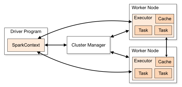
| Executor | one JVM per container | Runs tasks and holds cached blocks. Lives for the application, not the job |
| Job | one per action, such as count() |
An action triggers a job. Transformations alone build a plan and run nothing |
| Stage | the boxes in the Spark UI DAG | A run of tasks with no shuffle between them. A new stage starts at every shuffle boundary |
| Task | one per partition, per stage | The unit of work sent to an executor slot. 200 partitions means 200 tasks |
| Partition | df.rdd.getNumPartitions() |
The unit of parallelism. Too few starves the cluster, too many drowns it in scheduling |
| Shuffle | groupBy, join, repartition |
Redistributes data across executors over the network. The expensive thing you are usually tuning around |
| Slot | spark.executor.cores per executor |
How many tasks one executor runs at once. Total parallelism is executors times cores |
Adapted from the Apache Spark documentation.
flowchart LR
  subgraph ST1["stage 1: narrow, no shuffle"]
    direction LR
    R1["read trips"] --> F["filter, select"]
  end

  subgraph ST2["stage 2: after the shuffle"]
    direction LR
    AG["aggregate"] --> W["write, the action"]
  end

  F -->|"shuffle<br/>groupBy city_id"| AG
Everything between two shuffles is one stage, and a stage runs one task per partition. That is the whole scheduling model, and it is why “how many partitions” is the question behind most tuning.
Transformations are lazy and actions are eager. filter, select, join and
withColumn add to a plan; count, collect, show and write execute it.
Narrow against wide is the distinction that predicts everything else. A narrow transformation needs only the partition in front of it, so it runs in place. A wide one needs rows from other partitions, so it forces a shuffle, and a shuffle is what ends a stage.
flowchart TB
  subgraph NW["narrow: each output partition reads one input partition"]
    direction LR
    N1["p1"] --> N1b["p1'"]
    N2["p2"] --> N2b["p2'"]
    N3["p3"] --> N3b["p3'"]
  end

  subgraph WD["wide: each output partition reads many input partitions"]
    direction LR
    W1["p1"] --> X1["p1'"]
    W1 --> X2["p2'"]
    W2["p2"] --> X1
    W2 --> X2
    W3["p3"] --> X1
    W3 --> X2
  end

  NW ~~~ WD
| Kind | Operations | What it costs |
|---|---|---|
| Narrow | map, filter, select, withColumn, union, mapPartitions, coalesce |
Nothing beyond the work itself. No network, no stage boundary |
| Wide | groupBy, reduceByKey, join, distinct, repartition, sortBy, window functions |
A shuffle: write to disk, transfer over the network, read back. Ends the stage |
Two consequences worth holding on to. Counting the wide transformations in your job tells you how many stages it will have, which is the fastest way to predict a plan before running it. And a broadcast join is valuable precisely because it turns a wide transformation into a narrow one: the small side goes to every executor, so no rows have to move.
coalesce sits on the narrow side, which is exactly why it can starve upstream
parallelism: avoiding the shuffle means the reduced partition count propagates
backwards up the DAG.
That is why a typo in a filter often surfaces at the write, several lines
later.
Worked example: counting jobs, stages and tasks
Reading the counts off a piece of code is the skill this all builds to. Take this, on a table that reads as 8 input partitions:
from pyspark.sql.functions import col, when

trips = spark.read.parquet("s3a://lakehouse-prod/warehouse/trips")
# input partitions come from split size, not file count: check, do not assume
print(trips.rdd.getNumPartitions())                                  # say it is 8

by_city = (trips
    .filter(col("fare_amount") > 50)                                 # narrow
    .withColumn("fare_band",
                when(col("fare_amount") > 100, "high").otherwise("mid"))  # narrow
    .groupBy("city_id").count())                                     # WIDE: shuffle

by_city.write.parquet("s3a://lakehouse-prod/warehouse/trips_by_city")  # action
| Level | Count | Why |
|---|---|---|
| Jobs | 1 | One action, write. Actions are what trigger jobs |
| Stages | 2 | One wide transformation, groupBy, so one shuffle boundary |
| Tasks in stage 1 | 8 | One per input partition. The filter and withColumn fuse into the same tasks |
| Tasks in stage 2 | 200 | One per post-shuffle partition, from spark.sql.shuffle.partitions, unless AQE coalesces them |
The rules underneath are short enough to memorise. Jobs equal actions. Stages equal wide transformations plus one. Tasks equal partitions, per stage. Narrow transformations never add a stage; they fuse into the tasks of the stage they sit in, which is also what whole-stage code generation collapses into a single generated method.
Watch for two things that break the arithmetic. Some operations hide an extra
job: show() may run one job to peek and another to finish, and any operation
that needs to sample or infer, such as reading JSON without a schema or a
sortBy computing range boundaries, runs its own job first. And with adaptive
execution on, the 200 in stage 2 is an upper bound rather than the number you
will see, because coalescing runs after the shuffle statistics arrive.
3. RDD, DataFrame and Dataset
| API | Example | Description |
|---|---|---|
| RDD | sc.textFile("s3a://lakehouse-prod/raw/trips/").map(lambda l: l.split(",")) |
A distributed collection of objects with no schema. You control the partitioning and the functions; Catalyst cannot see inside them |
| DataFrame | spark.read.parquet(path).filter("fare_amount > 50") |
A Dataset[Row]: rows with a known schema. The optimizer can reorder, prune and push down. The default choice |
| Dataset | ds.filter(t => t.fare > 50) (Scala, Java) |
Typed rows of a case class. Compile-time type safety plus the optimizer, at the cost of some serialisation overhead |
| Dimension | RDD | DataFrame | Dataset |
|---|---|---|---|
| Schema | None | Yes, at runtime | Yes, plus compile-time types |
| Optimized by Catalyst | No | Yes | Yes |
| Tungsten binary format | No | Yes | Partly: typed lambdas fall back to objects |
| Type errors caught | Runtime | Runtime for column names | Compile time |
| Languages | Scala, Java, Python, R | Scala, Java, Python, R | Scala, Java only |
| Use it for | Unstructured data, custom partitioning, low-level control | Almost everything | Typed domain logic where compile-time safety earns its cost |
In Python, Dataset does not exist as a separate API: DataFrame is the typed
and untyped API at once, because Python has no compile-time type checking to
offer. In Scala, DataFrame is literally the alias Dataset[Row].
The practical rule is to stay in DataFrame or SQL. Every time you drop into an RDD or a typed lambda, Catalyst loses visibility into what you are doing and can no longer reorder, prune or generate code across that step. Reach for an RDD when you genuinely need something the structured API cannot express, not by habit.
4. RDD operations
Two kinds, and the distinction is the whole execution model: transformations build a plan lazily, actions run it.
| Transformation | Example | Description |
|---|---|---|
map(func) |
rdd.map(lambda x: x * 2) |
One output element per input element |
filter(func) |
rdd.filter(lambda x: x > 10) |
Keeps elements where func returns true |
flatMap(func) |
rdd.flatMap(lambda l: l.split(" ")) |
Zero or more output items per input item |
mapPartitions(func) |
rdd.mapPartitions(batch_fn) |
Runs once per partition. Use it to amortise a per-partition setup such as a database connection |
mapPartitionsWithIndex(func) |
rdd.mapPartitionsWithIndex(fn) |
The same, with the partition index |
sample(withReplacement, fraction, seed) |
rdd.sample(False, 0.1, 42) |
A random fraction |
union(other) |
a.union(b) |
All elements of both. No shuffle |
intersection(other) |
a.intersection(b) |
Elements in both. Shuffles |
distinct([numPartitions]) |
rdd.distinct() |
Deduplicates. Shuffles |
groupByKey([numPartitions]) |
pairs.groupByKey() |
(K, Iterable<V>). Shuffles everything, so prefer a reducing variant |
reduceByKey(func) |
pairs.reduceByKey(add) |
Combines per key, on the map side first. Much cheaper than groupByKey |
aggregateByKey(zero)(seqOp, combOp) |
Like reduceByKey but the result type can differ from the value type |
|
sortByKey([ascending]) |
pairs.sortByKey() |
Sorts by key. Shuffles |
join(other) |
a.join(b) |
(K, (V, W)) for keys present in both |
cogroup(other) |
a.cogroup(b) |
(K, (Iterable<V>, Iterable<W>)). The primitive the joins are built on |
cartesian(other) |
a.cartesian(b) |
Every pair. Quadratic, so treat with suspicion |
pipe(command) |
rdd.pipe("my_script.sh") |
Streams each partition through an external process |
coalesce(n) |
rdd.coalesce(10) |
Fewer partitions without a full shuffle |
repartition(n) |
rdd.repartition(200) |
Any partition count, with a full shuffle |
repartitionAndSortWithinPartitions(p) |
Repartition and sort in one pass. Cheaper than doing both separately |
| Action | Example | Description |
|---|---|---|
reduce(func) |
rdd.reduce(add) |
Aggregates to a single value with a commutative, associative function |
collect() |
rdd.collect() |
Brings everything to the driver. The classic driver OOM |
count() |
rdd.count() |
Number of elements |
first() |
rdd.first() |
The first element |
take(n) |
rdd.take(10) |
The first n elements |
takeSample(withReplacement, num) |
rdd.takeSample(False, 100) |
A random sample, to the driver |
takeOrdered(n, [ordering]) |
rdd.takeOrdered(10) |
The smallest n, by natural or custom order |
saveAsTextFile(path) |
rdd.saveAsTextFile(path) |
One file per partition |
saveAsSequenceFile(path) |
Hadoop SequenceFile. Java and Scala | |
saveAsObjectFile(path) |
Java serialisation. Java and Scala | |
countByKey() |
pairs.countByKey() |
A map of key to count, to the driver |
foreach(func) |
rdd.foreach(send) |
Runs a function for its side effects. Use foreachPartition to amortise setup |
Two habits worth forming. Prefer reduceByKey over groupByKey, because it
combines on the map side and shuffles far less. And treat every action that
returns data to the driver (collect, take, countByKey) as a driver memory
question, not a cluster one.
5. spark-submit
SparkPi ships with every distribution, so this runs as pasted on any cluster
and is the fastest way to prove a submit configuration works before pointing it
at your own jar:
spark-submit \
  --master yarn \
  --deploy-mode cluster \
  --name spark-pi \
  --class org.apache.spark.examples.SparkPi \
  --num-executors 20 \
  --executor-cores 4 \
  --executor-memory 16g \
  --driver-memory 8g \
  --conf spark.sql.shuffle.partitions=400 \
  $SPARK_HOME/examples/jars/spark-examples_2.13-4.1.3.jar \
  1000
The trailing 1000 is the application’s own argument, not Spark’s: SparkPi
reads it as the number of slices to parallelise across.
| Flag | Example | Description |
|---|---|---|
--master |
yarn, k8s://https://..., local[*] |
Which cluster manager to talk to |
--deploy-mode |
cluster or client |
cluster runs the driver inside the cluster; client runs it where you typed the command |
--num-executors |
20 |
Static executor count. Ignored when dynamic allocation is on |
--executor-cores |
4 |
Slots per executor. Concurrent tasks contend for the same HDFS client, so raising this has a ceiling |
--executor-memory |
16g |
Heap per executor. Default 1g, which is almost never what you want |
--driver-memory |
8g |
Driver heap. Default 1g. Raise it if you collect or broadcast large data |
--jars |
/opt/jars/postgresql-42.7.3.jar |
Extra jars on the classpath of driver and executors |
--packages |
org.apache.hudi:hudi-spark3.5-bundle_2.12:1.2.0 |
Maven coordinates, resolved at submit time |
--files |
/etc/app/log4j2.properties |
Files shipped to every working directory |
--conf |
spark.sql.shuffle.partitions=400 |
Any Spark property. Repeatable |
Dynamic allocation is deliberately absent above, because it and --num-executors
are mutually exclusive: turning on spark.dynamicAllocation.enabled makes the
fixed count irrelevant. If you want it, drop --num-executors, set
spark.dynamicAllocation.minExecutors and maxExecutors, and give it either an
external shuffle service or spark.dynamicAllocation.shuffleTracking.enabled.
Cluster mode against client mode decides where the driver runs, and that decides more than it sounds like.
flowchart TB
  subgraph CL["cluster mode: driver runs inside the cluster"]
    direction LR
    C1["spark-submit<br/>from a gateway"] --> C2["cluster manager"]
    C2 --> C3["driver<br/>in a container"]
    C3 --> C4["executors"]
    C1 -.->|"can disconnect"| C3
  end

  subgraph CI["client mode: driver runs where you submitted"]
    direction LR
    I1["spark-submit<br/>driver lives here"] --> I2["cluster manager"]
    I2 --> I3["executors"]
    I1 -->|"driver traffic"| I3
    I1 -.->|"kill this and<br/>the job dies"| I3
  end

  CL ~~~ CI
| Cluster mode | Client mode | |
|---|---|---|
| Driver runs | In a container the cluster manager allocates | In the spark-submit process |
| Submitting machine | Can disconnect once the job is accepted | Must stay up for the whole job |
| Driver logs | Through the cluster manager or history server | Straight to your terminal |
| Network | Driver and executors are both inside the cluster | Executors call back out to your machine |
| Use it for | Production and scheduled jobs | Interactive work, notebooks, spark-shell |
The one that bites: an interactive session is client mode, so the driver is on
the machine you are sitting at. A collect() that works in production can
exhaust the driver heap on your laptop, and closing the laptop kills the job.
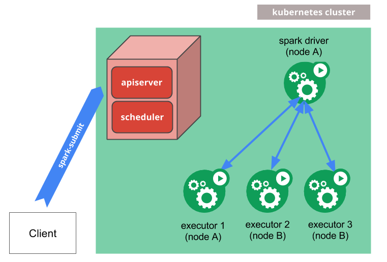
On Kubernetes the same roles map onto pods, with the driver pod creating and owning the executor pods:
Adapted from the Apache Spark documentation.
Note: Arguments after the application jar go to your
main, not to Spark. Anything Spark-facing must come before the jar. Options after it are passed to your application instead.
6. Memory model
| Concept | Config | Default | Description |
|---|---|---|---|
| Executor heap | spark.executor.memory |
1g |
The JVM heap. Minimum accepted is 450m |
| Executor overhead | spark.executor.memoryOverhead |
384m |
Off-heap: VM overhead, interned strings, native libraries |
| Overhead factor | spark.executor.memoryOverheadFactor |
0.10 |
Used instead of the flat value when larger. 0.40 for Kubernetes non-JVM jobs |
| Driver heap | spark.driver.memory |
1g |
Raise before you collect |
| Unified pool | spark.memory.fraction |
0.6 |
Share of (heap minus 300 MB reserved) available for execution plus storage |
| Storage floor | spark.memory.storageFraction |
0.5 |
The part of the unified pool that caching can hold against eviction |
| Cores per executor | spark.executor.cores |
1 |
Concurrent tasks per executor. Each task shares the same heap |
flowchart TB
  C["container the cluster manager allocates"] --> H["spark.executor.memory<br/>JVM heap"]
  C --> O["spark.executor.memoryOverhead<br/>off-heap, 384m or 10 percent"]
  H --> RES["reserved<br/>300 MB"]
  H --> UP["unified pool<br/>memory.fraction 0.6"]
  H --> USR["user memory<br/>the remaining 0.4"]
  UP --> EX["execution<br/>shuffles, joins, sorts"]
  UP --> ST["storage<br/>cached blocks<br/>floor at storageFraction 0.5"]
  %% execution can evict storage down to the floor; storage can never evict execution
  EX -.->|"evicts"| ST
The container your cluster manager sees is spark.executor.memory plus
overhead, so a 16g executor with the default factor asks for about 17.6g. When
a job is killed for exceeding its container limit and the heap looked fine, the
overhead is the first thing to check.
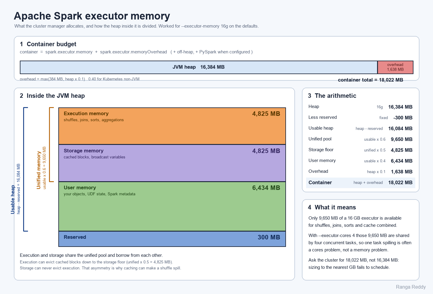
The bands are drawn in proportion to each other, except reserved memory, which is 1.8% of the heap and is given a minimum height so it can be labelled.
Worked example, --executor-memory 16g on the defaults. The formula is in
UnifiedMemoryManager: subtract the reserved 300 MB, then take
spark.memory.fraction of what is left.
| Step | Arithmetic | Result |
|---|---|---|
| Executor heap | --executor-memory 16g |
16384 MB |
| Less reserved system memory | 16384 − 300 | 16084 MB usable |
| Unified pool | 16084 × 0.6 | 9650 MB |
| Storage floor, protected from eviction | 9650 × 0.5 | 4825 MB |
| User memory, for your own objects | 16084 × 0.4 | 6434 MB |
| Off-heap overhead | max(384 MB, 16384 × 0.10) | 1638 MB |
| What the cluster manager must allocate | 16384 + 1638 | 18022 MB, about 17.6 GB |
Three things fall out of that arithmetic. Only about 9.4 GB of a 16 GB executor
is available for shuffles, joins, sorts and cache combined, which is less
than the container is given. The container is 10 percent larger than the heap
you
asked for, so a cluster sized to the nearest gigabyte will fail to schedule. And
with --executor-cores 4, those 9650 MB are shared by four concurrent tasks, so
one task spilling is often a cores-per-executor problem rather than a
memory-per-executor one.
The minimum is enforced: spark.executor.memory below 450 MB is rejected,
because the reserved 300 MB times 1.5 is the floor UnifiedMemoryManager
requires.
Execution memory (shuffles, joins, sorts) and storage memory (cached blocks) share one pool and borrow from each other. Execution can evict cached blocks down to the storage floor; storage can never evict execution. That is why caching a large DataFrame can quietly make a shuffle-heavy stage spill.
7. Reading and writing
| Operation | Example | Description |
|---|---|---|
| Read Parquet | spark.read.parquet("s3a://lakehouse-prod/raw/trips/") |
Schema comes from the footer. No inference pass |
| Read CSV with schema | spark.read.schema(s).csv(path) |
Always supply a schema. Inference reads the file twice |
| Read JSON | spark.read.json(path) |
Inference scans everything; supply a schema in production |
| Read JDBC | .option("partitionColumn","id").option("numPartitions","8") |
Without a partition column the whole table arrives on one task |
| Write partitioned | df.write.partitionBy("city_id").parquet(path) |
Directory-per-value. Keep cardinality low |
| Overwrite one partition | spark.sql.sources.partitionOverwriteMode=dynamic |
Default is STATIC, which wipes the whole table on overwrite. This is a data-loss footgun |
| Control output files | df.repartition(200).write... |
One output file per partition at write time |
| Max split size | spark.sql.files.maxPartitionBytes |
128MB default. Sets how large an input partition gets |
| Open cost | spark.sql.files.openCostInBytes |
4MB default. Estimated cost of opening a file, used to pack small files together |
# The single most useful read option for JDBC: parallelism
trips = (spark.read.format("jdbc")
    .option("url", "jdbc:postgresql://db.internal:5432/rides")
    .option("dbtable", "public.trips")
    .option("user", "etl")
    # partitionColumn must be numeric, date or timestamp. A string key will not do.
    .option("partitionColumn", "trip_seq")
    .option("lowerBound", "1")
    .option("upperBound", "40000000")
    .option("numPartitions", "16")
    .load())
Note:
spark.sql.sources.partitionOverwriteModedefaults toSTATIC, soINSERT OVERWRITEon a partitioned table replaces every partition, not just the ones in your DataFrame. Set it todynamicfor partition-scoped overwrites.
8. The Catalyst optimizer
Catalyst is why a DataFrame beats hand-written RDD code: you declare what you want and it decides how. Every query passes through four phases, each defined as rules over a tree.
flowchart TB
  SQL["SQL query<br/>or DataFrame code"] --> PARSE["parser"]
  PARSE --> UL["unresolved logical plan<br/><i>relations and columns are just names</i>"]

  UL --> AN["<b>Analyzer</b><br/>resolve against the catalog"]
  AN --> AL["analyzed logical plan<br/><i>every column typed and bound</i>"]
  AN -.->|"name not found"| ERR["AnalysisException"]
  CAT[("catalog<br/>tables, views,<br/>functions")] -.-> AN

  AL --> OPT["<b>Optimizer</b><br/>rule batches to fixed point"]
  OPT --> OL["optimized logical plan"]
  OPT -.- R1["predicate pushdown"]
  OPT -.- R2["column pruning"]
  OPT -.- R3["constant folding"]
  OPT -.- R4["limit pushdown"]
  OPT -.- R5["boolean simplification"]

  OL --> PLAN["<b>SparkPlanner</b><br/>strategies produce candidates"]
  PLAN --> PP["one or more<br/>physical plans"]
  STATS[("statistics<br/>sizes, row counts")] -.-> PLAN
  PP --> PICK["cost model selects one"]
  PICK --> SP["selected physical plan<br/><i>join strategy now fixed</i>"]

  SP --> CG["<b>WholeStageCodegenExec</b><br/>fuse operators into one Java method"]
  CG --> RDD["RDD[InternalRow]<br/>executed on the cluster"]

  RDD -.->|"real runtime statistics"| AQE["<b>AdaptiveSparkPlanExec</b><br/>re-plan the next stage"]
  AQE -.-> PLAN
The dashed loop at the bottom is the part that changed Spark 3 onwards: after a stage finishes, adaptive execution feeds its real statistics back into planning, so the join strategy and partition count for the next stage are chosen from measured sizes rather than estimates.
| Phase | Class | What it does |
|---|---|---|
| Analysis | Analyzer |
Resolves column and table names against the catalog, assigns types, and fails on anything unresolvable |
| Logical optimization | Optimizer |
Rule-based rewrites on the resolved tree: predicate pushdown, column pruning, constant folding, boolean simplification, limit pushdown |
| Physical planning | SparkPlanner |
Turns each logical operator into one or more physical candidates, such as picking a join strategy, then selects between them |
| Code generation | WholeStageCodegenExec |
Collapses a chain of operators into a single generated Java method, removing virtual calls and intermediate rows |
| Concept | Example | Description |
|---|---|---|
| Rule executor | RuleExecutor |
Applies rule batches to fixed point or a set number of iterations. Every phase above is built on it |
| Predicate pushdown | filter moved below a join or into the scan | The highest-value rewrite. Check it happened rather than assume it |
| Column pruning | only the projected columns read | Why SELECT * on a wide Parquet table costs so much more than naming columns |
| Constant folding | WHERE 1 = 1 removed |
Evaluates at plan time |
| Cost-based optimization | spark.sql.cbo.enabled, default false |
Uses table statistics to reorder joins. Needs ANALYZE TABLE ... COMPUTE STATISTICS first |
| Adaptive re-planning | AdaptiveSparkPlanExec |
Re-runs parts of planning mid-query using real statistics. The subject of the AQE section below |
| Inspect the result | df.explain("formatted") |
formatted, extended, cost or codegen. extended prints all four phases |
-- See every phase for a query, which is the fastest way to learn what Catalyst did
EXPLAIN EXTENDED
SELECT c.city_name, count(*)
FROM trips t JOIN cities c ON t.city_id = c.city_id
WHERE t.fare_amount > 50
GROUP BY c.city_name;
The reason this matters in practice: Catalyst can only optimise what it can see. A SQL expression or a DataFrame column expression is a tree it can rewrite. A Python UDF or an RDD lambda is an opaque function it must call as-is, which blocks pushdown across that point. That is the real cost of a UDF, and it is usually larger than the cost of the function itself.
9. Joins
| Strategy | Hint | Description |
|---|---|---|
| Broadcast hash join | /*+ BROADCAST(d) */ |
Ships the small side to every executor. No shuffle. The fastest option when one side fits |
| Shuffle hash join | /*+ SHUFFLE_HASH(a, b) */ |
Shuffles both sides, builds a hash table on one. Good when one side is much smaller but too big to broadcast |
| Sort merge join | /*+ MERGE(a, b) */ |
Shuffles and sorts both sides. The default for large-to-large joins |
| Broadcast nested loop | /*+ SHUFFLE_REPLICATE_NL(a, b) */ |
The fallback for non-equi joins. Quadratic, so watch it |
| Concept | Example | Description |
|---|---|---|
| Broadcast threshold | spark.sql.autoBroadcastJoinThreshold |
10MB default. Raise it when the small side is well-known and stats are reliable |
| Disable broadcast | set the threshold to -1 |
Useful when a bad size estimate keeps broadcasting something large and OOMing the driver |
| AQE broadcast threshold | spark.sql.adaptive.autoBroadcastJoinThreshold |
No static default; falls back to the non-AQE threshold. Applies using runtime sizes |
| Join hint in SQL | SELECT /*+ BROADCAST(cities) */ ... |
Hints go right after SELECT |
| Join hint in Python | trips.join(broadcast(cities), "city_id") |
from pyspark.sql.functions import broadcast |
SELECT /*+ BROADCAST(c) */ t.trip_id, t.fare_amount, c.city_name
FROM trips t JOIN cities c ON t.city_id = c.city_id;
The join that hurts is the one where both sides are large and the key is skewed. AQE handles the common case automatically; see the skew settings below.
10. Shuffle and partitioning
| Operation | Example | Description |
|---|---|---|
repartition(n) |
df.repartition(200) |
Full shuffle to exactly n partitions. Use to increase parallelism or even out skew |
repartition(col) |
df.repartition("city_id") |
Hash-partition by column. Co-locates a key before a join or a write |
coalesce(n) |
df.coalesce(10) |
Merges partitions without a full shuffle. Cheap, but can starve upstream parallelism |
partitionBy |
df.write.partitionBy("dt") |
A write-time directory layout, unrelated to repartition |
| Shuffle partitions | spark.sql.shuffle.partitions |
200 default since 1.1.0. The post-shuffle partition count when AQE is not coalescing |
| Default parallelism | spark.default.parallelism |
RDD-level default. Ignored by DataFrame shuffles |
The coalesce trap is worth spelling out: df.repartition(1000).coalesce(1)
does not give you 1000-way parallelism then one file. Because coalesce avoids
the shuffle, it pushes the narrow partition count up the DAG, and the upstream
work runs with one task. Use repartition(1) when you genuinely want the shuffle.
11. Adaptive query execution
AQE re-optimises the plan mid-flight using statistics from completed stages, which is why it beats anything you can set by hand ahead of time.
flowchart LR
  P["logical plan"] --> ST1["run stage 1"]
  ST1 --> STATS["real statistics<br/>partition sizes, row counts"]
  STATS --> RE["re-optimise"]
  RE --> C1["coalesce small<br/>partitions"]
  RE --> C2["split skewed<br/>partitions"]
  RE --> C3["switch sort merge<br/>to broadcast"]
  C1 --> ST2["run stage 2"]
  C2 --> ST2
  C3 --> ST2
| Feature | Config | Default | Description |
|---|---|---|---|
| Enable AQE | spark.sql.adaptive.enabled |
true |
On by default since 3.2 |
| Coalesce partitions | spark.sql.adaptive.coalescePartitions.enabled |
true |
Merges small post-shuffle partitions, so an over-large shuffle.partitions stops mattering |
| Advisory size | spark.sql.adaptive.advisoryPartitionSizeInBytes |
64MB |
The post-shuffle partition size AQE aims for |
| Minimum size | spark.sql.adaptive.coalescePartitions.minPartitionSize |
1MB |
Floor, so coalescing does not produce tiny partitions |
| Skew join handling | spark.sql.adaptive.skewJoin.enabled |
true |
Splits oversized partitions on the skewed side |
| Skew factor | spark.sql.adaptive.skewJoin.skewedPartitionFactor |
5.0 |
A partition is skewed at this multiple of the median |
| Skew threshold | spark.sql.adaptive.skewJoin.skewedPartitionThresholdInBytes |
256MB |
And it must also exceed this absolute size |
| Local shuffle reader | spark.sql.adaptive.localShuffleReader.enabled |
true |
Avoids a network fetch when a sort merge join becomes a broadcast join |
Both skew conditions must hold: a partition is treated as skewed only when it is larger than 5 times the median and larger than 256 MB. On a job whose partitions are all under 256 MB, skew handling never fires no matter how uneven they are. That is worth checking before concluding skew handling is broken.
12. Caching and persistence
| Storage level | Available in | Description |
|---|---|---|
MEMORY_ONLY |
all | Deserialized objects in the JVM. Partitions that do not fit are recomputed on each use. The default for rdd.cache() |
MEMORY_AND_DISK |
all | Deserialized in memory; partitions that do not fit spill to disk and are read back. The default for df.cache() |
MEMORY_ONLY_SER |
Java, Scala | Serialized, one byte array per partition. More space-efficient, more CPU to read |
MEMORY_AND_DISK_SER |
Java, Scala | Like MEMORY_ONLY_SER, but spills to disk instead of recomputing |
DISK_ONLY |
all | Partitions on disk only |
MEMORY_ONLY_2, MEMORY_AND_DISK_2, DISK_ONLY_2 |
all | The same levels, replicated on two nodes. Rebuild from the replica instead of recomputing when a node is lost |
DISK_ONLY_3 |
all | Disk, replicated three ways |
OFF_HEAP |
experimental | Like MEMORY_ONLY_SER but in off-heap memory, which must be enabled first |
Note: In Python, objects are always serialized with Pickle, so the
_SERlevels do not exist as a separate choice. The levels available from PySpark areMEMORY_ONLY,MEMORY_ONLY_2,MEMORY_AND_DISK,MEMORY_AND_DISK_2,DISK_ONLY,DISK_ONLY_2andDISK_ONLY_3.
The two defaults differ and it catches people: rdd.cache() is MEMORY_ONLY,
so anything that does not fit is silently recomputed every time. df.cache() is
MEMORY_AND_DISK, so it spills instead. If an RDD cache seems to do nothing,
that asymmetry is usually why.
| Operation | Example | Description |
|---|---|---|
| Cache at the default level | df.cache() |
Shorthand for persist() at the API’s default level |
| Choose a level | df.persist(StorageLevel.DISK_ONLY) |
from pyspark import StorageLevel |
| Release it | df.unpersist() |
Cached blocks compete with execution memory. Free them when the branch is done |
| Truncate lineage | df.checkpoint() |
Writes to reliable storage and drops the lineage. For very long or iterative plans |
| Lightweight variant | df.localCheckpoint() |
Truncates lineage using executor storage. Faster, but lost if an executor is lost |
| Inspect what is cached | Spark UI, Storage tab | Shows each cached dataset, its level, and the fraction actually in memory |
The documentation’s own selection order is worth following: stay on the default if the data fits; move to a serialized level to save space before you move to disk; and only spill to disk when recomputing would be more expensive than reading it back, which is the case when the computation was expensive or filtered a lot of data away.
Cache when a DataFrame is used more than once and producing it was expensive. Caching something read once makes the job slower, because you pay the write and give up memory that execution wanted.
13. Spark SQL and ANSI mode
The biggest behavioural change in the Spark 4 line is ANSI mode.
spark.sql.ansi.enabled now defaults to true, and the default is computed as
“true unless the SPARK_ANSI_SQL_MODE environment variable is set to false”.
| Behaviour | ANSI off, Spark 3 style | ANSI on, Spark 4 default |
|---|---|---|
| Integer overflow | Wraps silently | Raises an arithmetic overflow error |
| Divide by zero | Returns NULL |
Raises a divide-by-zero error |
CAST('abc' AS INT) |
Returns NULL |
Raises a cast error |
| Out-of-range store | Silently truncates or nulls | Rejected at analysis time |
| Concept | Example | Description |
|---|---|---|
| Turn ANSI off per session | SET spark.sql.ansi.enabled=false |
The quick unblock when an upgrade surfaces bad data |
| Turn it off cluster-wide | SPARK_ANSI_SQL_MODE=false |
The environment escape hatch the default reads |
| Safe cast | try_cast(x AS INT) |
Returns NULL instead of raising, without disabling ANSI globally |
| Safe arithmetic | try_divide(a, b), try_add(a, b) |
Per-expression opt-out. The better fix than a global switch |
| Store assignment | spark.sql.storeAssignmentPolicy |
ANSI. Governs what an INSERT will implicitly coerce |
| Cost-based optimiser | spark.sql.cbo.enabled |
false. Needs ANALYZE TABLE ... COMPUTE STATISTICS to be worth enabling |
Treat an ANSI failure on upgrade as a finding rather than a blocker: the error is
usually pointing at data that was silently becoming NULL before. Reach for
try_cast and try_divide at the specific expression before turning the flag
off everywhere.
14. Structured Streaming
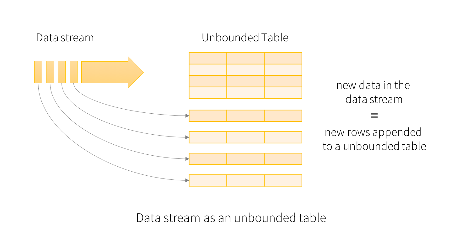
The model to hold in your head is that a stream is an unbounded table, with each arriving batch appended as new rows:
Adapted from the Apache Spark documentation.
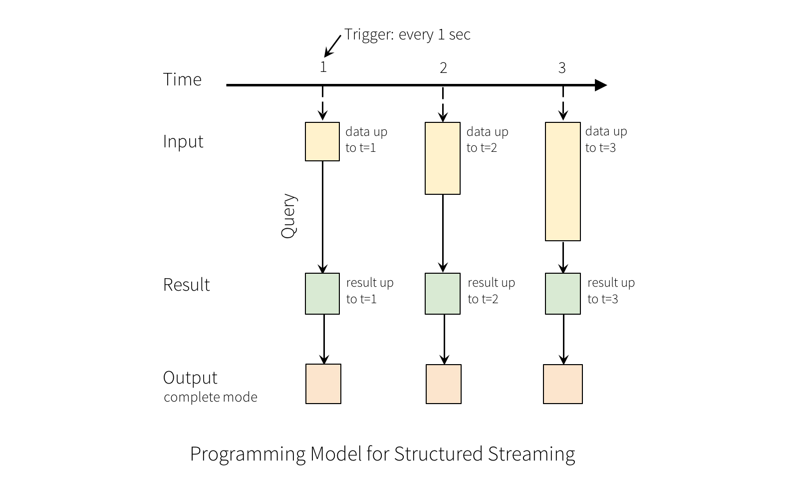
A query over that table produces a result table, recomputed incrementally each trigger, and the output mode decides which of its rows get written out:
Adapted from the Apache Spark documentation.
| Concept | Example | Description |
|---|---|---|
| Source | spark.readStream.format("kafka") |
Kafka, files, rate, socket. Same DataFrame API as batch |
| Sink | .writeStream.format("delta") |
Files, Kafka, foreachBatch, console, memory |
| Checkpoint | .option("checkpointLocation", path) |
Required for fault tolerance. One per query, never shared |
| Trigger: micro-batch | .trigger(processingTime="1 minute") |
Fixed cadence. The default is as fast as possible |
| Trigger: once | .trigger(availableNow=True) |
Process everything outstanding and stop. The batch-shaped way to run a stream |
| Output: append | .outputMode("append") |
New rows only. The default, and the only one many sinks accept |
| Output: update | .outputMode("update") |
Rows whose aggregate changed |
| Output: complete | .outputMode("complete") |
The whole result table every batch. Aggregations only |
| Watermark | .withWatermark("event_time", "10 minutes") |
How late an event may arrive. Bounds the state store |
| Arbitrary sink logic | .foreachBatch(fn) |
Gives you a batch DataFrame per micro-batch. How you write to a sink with no native connector |
from pyspark.sql.functions import col, from_json, window, count
from pyspark.sql.types import StructType, StringType, TimestampType, DoubleType

schema = (StructType()
    .add("trip_id", StringType())
    .add("city_id", StringType())
    .add("fare_amount", DoubleType())
    .add("started_at", TimestampType()))

events = (spark.readStream.format("kafka")
    .option("kafka.bootstrap.servers", "kafka-broker1:9092")
    .option("subscribe", "trips")
    .option("startingOffsets", "latest")
    .load()
    # Kafka's own `timestamp` is broker ingest time. Event time comes from the
    # payload, which is what a watermark should be based on.
    .select(from_json(col("value").cast("string"), schema).alias("t"))
    .select("t.*"))

# A plain pass-through sink: no state, so no watermark is needed.
(events.writeStream
    .format("parquet")
    .option("checkpointLocation", "s3a://lakehouse-prod/checkpoints/trips_raw")
    .option("path", "s3a://lakehouse-prod/warehouse/trips_raw")
    .trigger(processingTime="1 minute")
    .outputMode("append")
    .start())

# A stateful aggregation, which is where the watermark actually does work:
# it finalises windows and lets Spark drop their state.
(events
    .withWatermark("started_at", "10 minutes")
    .groupBy(window(col("started_at"), "5 minutes"), col("city_id"))
    .agg(count("*").alias("trips"))
    .writeStream
    .format("parquet")
    .option("checkpointLocation", "s3a://lakehouse-prod/checkpoints/trips_by_window")
    .option("path", "s3a://lakehouse-prod/warehouse/trips_by_window")
    .outputMode("append")
    .start())
The two queries above are deliberately different. A watermark on the first would be inert: it only has an effect on stateful operations, which a pass-through sink is not. Each query also gets its own checkpoint location, which is a hard requirement rather than a convention.
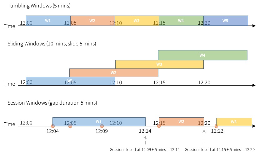
Event-time windows come in three shapes, and the choice changes how many windows a single record lands in:
Adapted from the Apache Spark documentation.
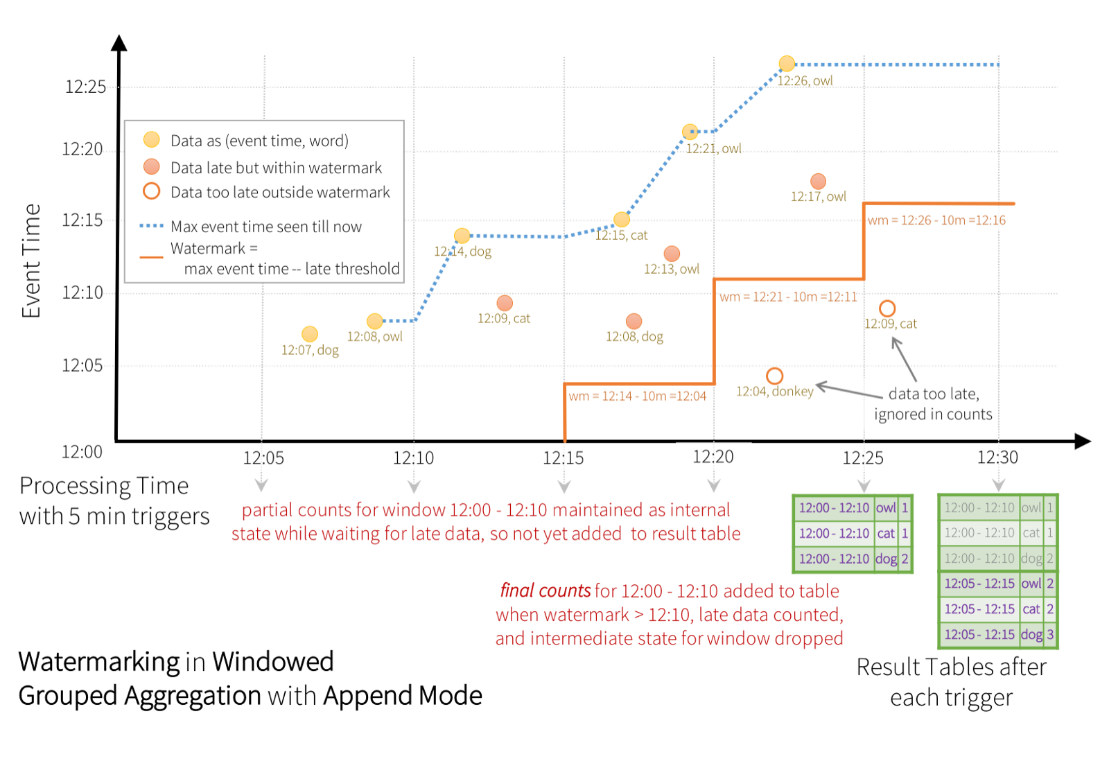
The watermark is what lets Spark finalise a window and drop its state. Anything arriving behind the watermark is too late to be counted:
Adapted from the Apache Spark documentation.
Without a watermark, a streaming aggregation keeps state forever and the job degrades over days rather than failing outright. The watermark is what lets Spark drop state it will never need again.
15. Useful functions and patterns
| Pattern | Example | Description |
|---|---|---|
| Window ranking | row_number().over(Window.partitionBy("city_id").orderBy(desc("fare"))) |
Deduplicate or top-N per group. One shuffle, unlike a self-join |
| Deduplicate by key | dropDuplicates(["trip_id"]) |
Keeps an arbitrary row. Use a window with an explicit order when which row wins matters |
| Explode arrays | select(explode("items").alias("item")) |
One output row per element |
| Pivot | groupBy("city_id").pivot("status").count() |
Supply the value list to avoid a pass that discovers it |
| Conditional | when(col("fare") > 50, "high").otherwise("low") |
The SQL CASE equivalent |
| Null-safe equality | col("a").eqNullSafe(col("b")) |
<=> in SQL. Treats null equal to null, unlike = |
| Coalesce nulls | coalesce(col("a"), col("b"), lit(0)) |
First non-null. Unrelated to DataFrame.coalesce |
| Salting a skewed key | concat(col("k"), lit("_"), (rand()*16).cast("int")) |
Spreads a hot key across partitions when AQE skew handling does not fire |
| Broadcast a small side | join(broadcast(dim), "city_id") |
Forces the strategy when statistics are unreliable |
| Inspect the plan | df.explain("formatted") |
formatted, extended or cost. The fastest way to check a pushdown |
from pyspark.sql import Window
from pyspark.sql.functions import row_number, desc, col

# Latest row per trip, which is the shape most CDC dedup takes
latest = (trips
    .withColumn("rn", row_number().over(
        Window.partitionBy("trip_id").orderBy(desc("updated_at"))))
    .where(col("rn") == 1)
    .drop("rn"))
16. Diagnosing a slow job
| Symptom | Where to look | Likely cause |
|---|---|---|
| A few tasks take far longer than the rest | Stage page, task duration percentiles | Skew. Check AQE skew thresholds, or salt the key |
| Huge spill to disk | Stage page, spill columns | Partitions too large. Raise parallelism or lower the advisory size |
| Thousands of tiny tasks | Stage page, task count and median duration | Over-partitioned input, or too many small files |
| Driver out of memory | Driver logs | A collect, or a broadcast of something much larger than estimated |
| Container killed, heap looked fine | Cluster manager logs | memoryOverhead too small for the workload |
| Stage retries repeatedly | Stage page, failure reason | Executor loss, often overhead or a shuffle fetch failure |
| Planning slower than execution | SQL tab, plan time | Too many files or partitions. Compact, or prune harder |
| Reads scan everything | SQL tab, physical plan | Predicate not pushed down. Check the filter is on a partition or statistics column |
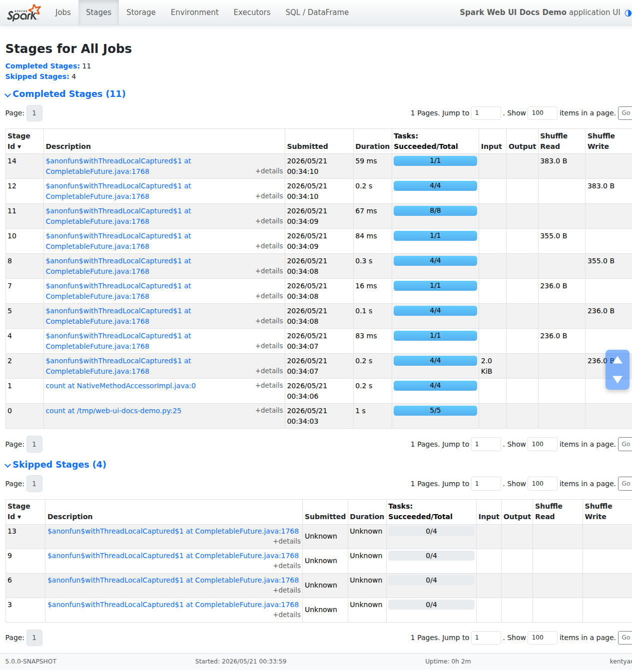
The stages page is where skew and spill show up, because it gives you the task duration percentiles rather than just an average:
Source: Apache Spark documentation.
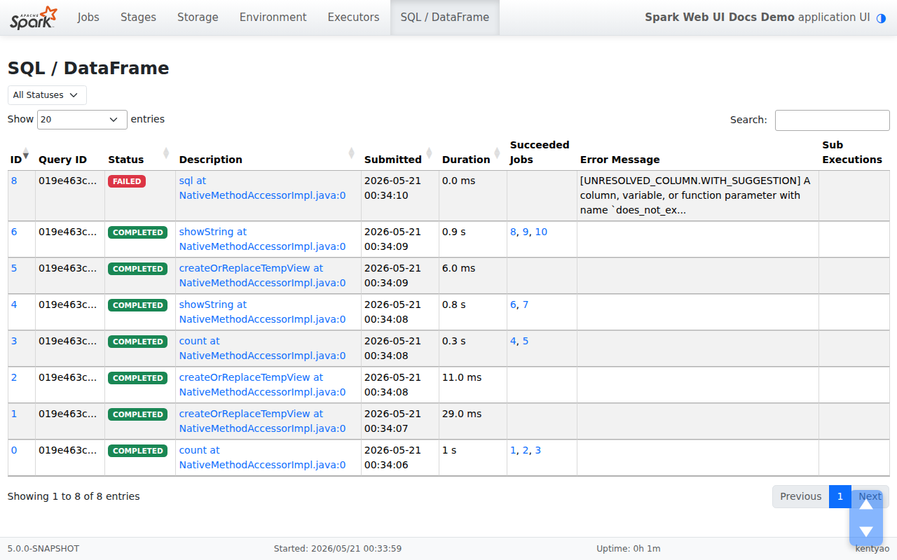
And the SQL tab lists each query with its duration and plan:
Source: Apache Spark documentation.
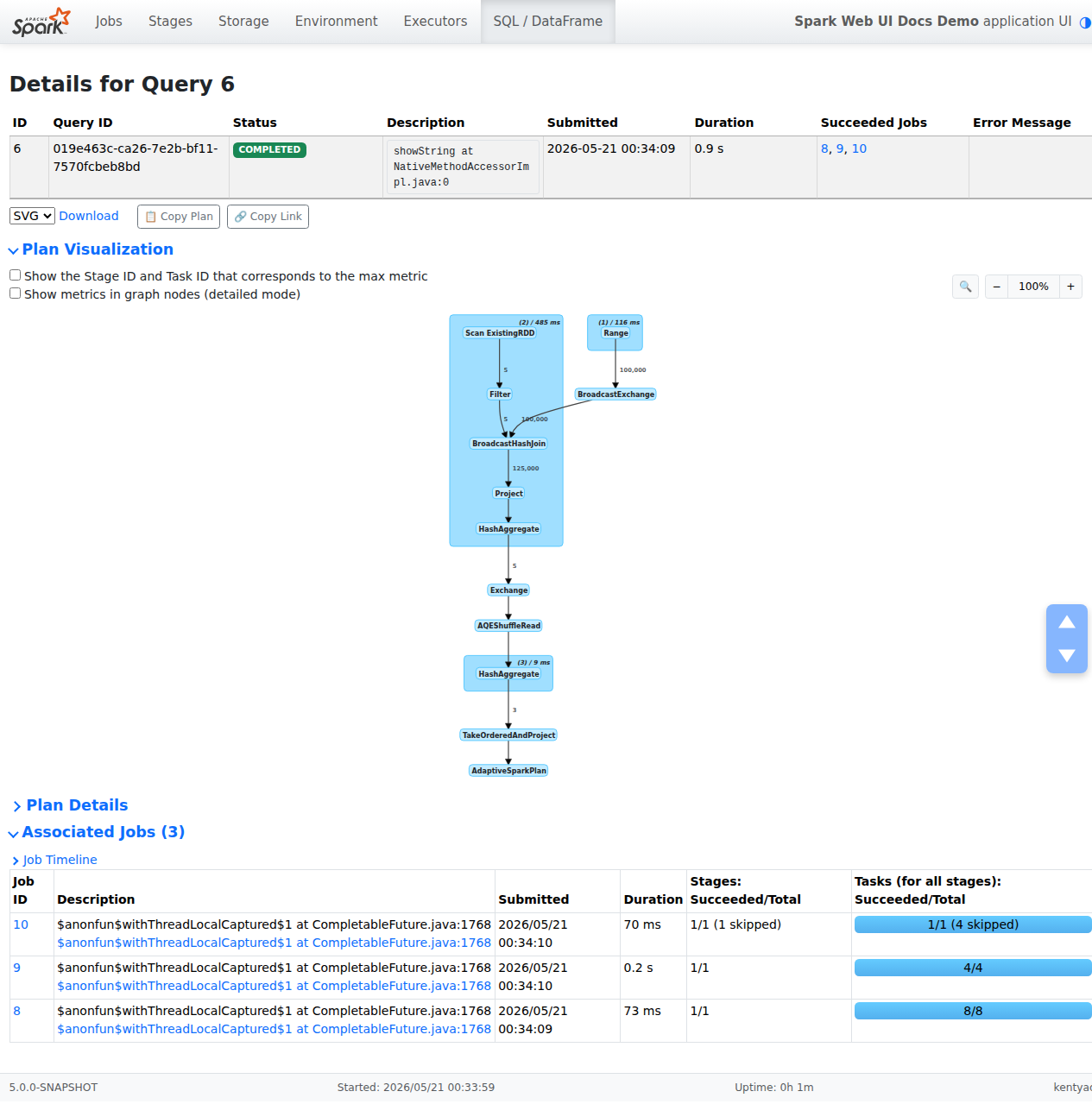
Opening one gives you the physical plan annotated with row counts per node, which answers “did my filter push down” and “which side got broadcast” directly:
Source: Apache Spark documentation.
The Spark UI SQL tab is the most useful page and the least used. It shows the physical plan with row counts per node, which answers “did my filter push down” and “which side got broadcast” directly, rather than by inference.
17. Upgrading to Spark 4
Section 1 lists what arrived. This is what breaks, which is a shorter and more useful list.
| What breaks | Why | What to do |
|---|---|---|
| Queries that relied on silent nulls | ANSI mode turns a bad cast, an overflow and a divide by zero into runtime errors | Fix the expression with try_cast or try_divide, rather than disabling ANSI globally |
INSERT with a lossy implicit coercion |
spark.sql.storeAssignmentPolicy is ANSI, so the coercion is rejected at analysis time |
Cast explicitly in the SELECT |
| Scala 2.12 builds | Spark 4 is Scala 2.13 only | Rebuild against 2.13; check every third-party jar has a 2.13 artifact |
| Java 8 and 11 runtimes | Spark 4 requires Java 17 or later | Move the cluster runtime before the Spark version |
| Pinned connector jars | Format bundles are built per Spark line | Take the bundle built for 4.x, for example a hudi-spark4.x-bundle |
-- The one-line rehearsal: run your suite on the OLD runtime with ANSI on.
-- Every failure here is a Spark 4 failure you can fix before upgrading.
SET spark.sql.ansi.enabled = true;
Doing that first splits the upgrade in two. ANSI failures are data and expression problems you can fix on the version you already run; everything else is runtime and dependency work. Meeting both at once is what makes a Spark 4 upgrade feel hard.
Conclusion
Most Spark tuning reduces to three questions: how many partitions, how large, and is the data evenly spread across them. Executor sizing and memory fractions matter, but they matter because they decide how much work a single task can hold before it spills.
Adaptive query execution has absorbed most of what used to be manual tuning. It
coalesces small partitions, splits skew and re-picks join strategies from real
statistics, which means spark.sql.shuffle.partitions is far less load-bearing
than the tuning guides of a few years ago suggest. Set it roughly and let AQE
adjust.
The one thing to plan for deliberately on the 4.x line is ANSI mode. It is a good default and it will surface data problems that the 3.x line hid, so give it a dedicated test pass rather than meeting it during an upgrade.
References
- Spark configuration reference for every property, its default and the version it appeared in
- SQL performance tuning for adaptive query execution, join hints and partition coalescing
- Structured Streaming programming guide for triggers, watermarks and output modes
- ANSI compliance for the full list of behaviours the Spark 4 default changes
- Apache Hudi on Spark: the complete cheat sheet for the lakehouse layer on top of this
Trademarks
Apache Spark, Apache Hudi, Apache Iceberg, Apache Kafka, Apache Parquet, Apache Hadoop, Apache Hive and Apache are either registered trademarks or trademarks of The Apache Software Foundation in the United States and other countries.
Found this useful?
These posts and tools are free. If one saved you an afternoon, you can buy me a coffee.