Sorting and clustering in Iceberg: what min/max statistics can and cannot skip
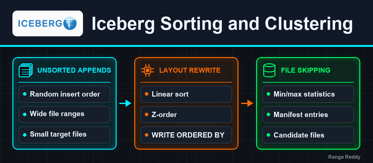
Iceberg skips a data file when its per-column min and max cannot contain your predicate. Which files it can skip is decided entirely by how the rows were laid out. Here is that measured: the same table and the same query going from 34 files scanned to 1, the secondary sort key that buys nothing, and a z-order that made the leading column no better than unsorted.
- How file skipping actually works
- Seeing the statistics
- The dataset
- Unsorted: nothing is skippable
- Linear sort: 34 candidates become 1
- The secondary sort key that buys nothing
- Z-order: a different trade, not a better sort
- Keeping it sorted without rewriting
- Sorting or partitioning?
- What it costs
- Common misconceptions
- Run it yourself
- Frequently asked questions
- Conclusion
- References
- Trademarks
TL;DR
- Iceberg prunes files using per-column min/max statistics. A file is skipped only when its range cannot contain your predicate, so pruning is a property of the layout, not of the query.
- On an unsorted table, every file’s
city_idrange spanned the whole domain, so acity_id = 42query had 34 of 34 files as candidates. Nothing was skippable.- Sorting by that column took it to 1 of 26. The average per-file range collapsed from 500 values to about 19.
- A secondary sort key buys almost no file-level pruning. Sorting by
(city_id, amount)left a narrowamountfilter reading 42 of 43 files, becauseamountis only ordered within eachcity_id.- Z-order is not a better sort, it is a different trade.
zorder(city_id, amount)madeamountprunable (1 of 47) and the leading column no better than unsorted (47 of 47). Measure before assuming it is the advanced option.- You do not have to rewrite to get this.
ALTER TABLE ... WRITE ORDERED BYmade a plain append land sorted: 1 of 19 candidate files instead of 18 of 18. A one-off sort decays: three unsorted appends took the same query from 1 candidate to 19.
A read query in Iceberg is a sequence of eliminations, and the last one — skipping individual data files using the statistics held in their manifest entry — only pays off if the rows were written in an order that makes those statistics narrow. That post says so and moves on. This one measures what “narrow” is worth.
The short version is that layout, not tuning, decides how much of a table a query has to read. And the gap between a good layout and no layout is not ten percent.
How file skipping actually works
For every data file, Iceberg stores the minimum and maximum value of each column
in the manifest entry that points at it. Planning a query is then arithmetic: for
a predicate city_id = 42, a file whose city_id range is [100, 180] cannot
contain a matching row, so it is never opened.
flowchart LR
    P["predicate<br/>city_id = 42"] --> M{"file range<br/>contains 42?"}
    M -->|no| S["skipped<br/>never opened"]
    M -->|yes| R["read<br/>and filtered"]
Two consequences follow, and they are the whole post:
- The statistic is per column, per file. It is a bounding box, not an index. It cannot express “this file contains city 42 and no others nearby”.
- A file whose range spans the whole domain is never skippable, whatever the predicate. Random insertion order produces exactly that.
Seeing the statistics
You do not have to infer any of this from timings. Iceberg exposes the numbers in
the files metadata table, and readable_metrics presents them already typed:
SELECT file_path,
       readable_metrics.city_id.lower_bound,
       readable_metrics.city_id.upper_bound
FROM   ice.blog_sorting.events.files;
Which makes “how many files could this query possibly need?” a query rather than a guess — count the files whose range brackets the value:
SELECT count(*) AS candidate_files
FROM   ice.blog_sorting.events.files
WHERE  readable_metrics.city_id.lower_bound <= 42
  AND  readable_metrics.city_id.upper_bound >= 42;
Every candidate count below comes from that query, and each one was checked
against the planner itself: the scan node’s resultDataFiles metric, the number
of data files Iceberg actually planned for the query, matched the candidate count
in every layout measured here. The query is the planner’s decision, readable
before you run anything.
The dataset
Two million rows, city_id drawn uniformly from 500 values and amount from
[0, 1000), written in random order: the shape you get from any ingestion that
appends as data arrives. The target file size is set small so the table has
enough files to be interesting on a laptop:
CREATE TABLE ice.blog_sorting.events (
  id BIGINT, city_id INT, amount DOUBLE, ts TIMESTAMP)
USING iceberg
TBLPROPERTIES ('write.target-file-size-bytes'='1048576');
city_id = 42 matches 3,986 rows of the two million: 0.2% of the table. A
perfect layout would read one file; a useless one reads all of them. The scripts
that build it and measure every layout are in
Run it yourself.
Unsorted: nothing is skippable
files = 34
candidate files for city_id = 42 = 34   (planned by the scan: 34)
average city_id range per file = 500 values (of 500 possible)
Every file contains a near-complete spread of city_id, because the rows arrived
in random order and each file is just a slice of that stream. The bounding box of
each file is the whole domain, so the predicate excludes nothing. The query reads
100% of the table to return 0.2% of it, and no amount of configuration
changes that.
This is the default state of any table that appends as data arrives.
Linear sort: 34 candidates become 1
rewrite_data_files with the sort strategy rewrites the table in a given order:
CALL ice.system.rewrite_data_files(
  table       => 'blog_sorting.events',
  strategy    => 'sort',
  sort_order  => 'city_id ASC NULLS LAST',
  options     => map('rewrite-all','true'));
files = 26
candidate files for city_id = 42 = 1   (planned by the scan: 1)
average city_id range per file = 19.3 values (of 500)
One file out of twenty-six. The mechanism is visible in the range: each file now
holds about nineteen adjacent city_id values instead of all five hundred, so a
single-value predicate falls inside exactly one file’s box.
The file count changed too, from 34 to 26, because the rewrite also re-packs rows to the target file size. It does not always go down: the two-column sort below wrote 43 files and the z-order 47, from the same 34. If you track file counts for another reason, measure after the rewrite rather than assuming compaction.
A sort rewrite samples the data to choose its ranges, so its exact file count and average range move slightly between runs: across two runs this layout wrote 26 and 25 files, with averages of 19.3 and 20.0. The candidate counts did not move.
The secondary sort key that buys nothing
The obvious next step is to sort by both columns, expecting both to become prunable. It does not work, and the reason is worth internalising:
sort_order => 'city_id ASC NULLS LAST, amount ASC NULLS LAST'
| Layout | files | avg city_id range (of 500) |
avg amount range (of 1000) |
files for amount 500–505 |
|---|---|---|---|---|
| Unsorted | 34 | 500.0 | 1000.0 | 34 of 34 |
city_id |
26 | 19.3 | 999.9 | 26 of 26 |
city_id, amount |
43 | 12.6 | 969.8 | 42 of 43 |
Adding amount as a secondary key barely changed its per-file range. It is
still almost the full domain, and a narrow amount filter still needed 42 of
the 43 files.
That is not a bug. amount is ordered only within each city_id, and a file
spans roughly thirteen different city_id values, so it contains thirteen
independent runs of amount, each starting near zero and ending near the
maximum. The file’s amount bounding box is therefore nearly the whole range,
and a bounding box is all the statistic can record. The one file skipped was one
whose rows happened to come from a single city_id.
A secondary sort key helps compression and row-group skipping inside a file. It does not help file-level pruning. If you need two columns prunable, linear sorting is the wrong tool.
Z-order: a different trade, not a better sort
Z-ordering interleaves the bits of several columns so that rows close in multiple dimensions end up close on disk. That is the standard answer to the problem above, so it is worth measuring rather than assuming:
sort_order => 'zorder(city_id, amount)'
| Layout | files | city_id = 42 candidates |
amount 500–505 candidates |
|---|---|---|---|
| Unsorted | 34 | 34 | 34 |
Linear city_id |
26 | 1 | 26 |
zorder(city_id, amount) |
47 | 47 | 1 |
Read the middle column twice. Z-ordering made the leading column need every
file, where the linear sort needed one: no better than not sorting at all. What
it bought was amount: from 26 candidates down to 1.
The per-column ranges say the same thing:
linear(city_id)          avg city range  19.3/500   avg amount range 999.9/1000
zorder(city_id, amount)  avg city range 500.0/500   avg amount range  21.3/1000
So the trade is explicit. A linear sort makes one column excellent and leaves the rest untouched. A z-order spreads the benefit, and in this case spread it so unevenly that the first column got nothing.
Why so lopsided? Iceberg’s z-order turns every column into an 8-byte,
order-preserving value (ZOrderByteUtils, PRIMITIVE_BUFFER_SIZE = 8) and then
interleaves the bits, most significant first. city_id is an INT from 0 to
499: widened to 8 bytes, its top 55 bits are the same in every row, and only the
last 9 vary. amount is a DOUBLE from 0 to 1000, and its exponent and leading
mantissa bits, at the top of the encoding, vary from row to row. The first bits
that differ between rows in the interleaved key are therefore all amount’s, so
the ordering came out as “sorted by amount”. What is measured above is the
effect; the encoding is the mechanism that produces it.
The practical rule that follows: z-order columns of comparable cardinality and type, and check the resulting ranges rather than trusting that it helped. If one column matters far more than the others, a linear sort on that column will beat z-order on it every time.
Keeping it sorted without rewriting
Everything above rewrote the table. You usually do not have to, because a table can declare the order it wants new writes to arrive in:
ALTER TABLE ice.blog_sorting.events WRITE ORDERED BY city_id ASC NULLS LAST;
Spark honours the declaration by default: once a table has a sort order, its
default write distribution is range (SparkWriteConf), so each write is
range-partitioned and sorted by the declared key before files are written. The
same million-row append, with and without it:
| files | avg city_id range |
candidates for city_id = 42 |
|
|---|---|---|---|
| Plain append | 18 | 500.0 | 18 |
WRITE ORDERED BY city_id |
19 | 27.2 | 1 |
One file instead of eighteen, from a declaration on the table rather than a maintenance job. The range is looser than the full rewrite achieved (27 values per file against 19) because each write only sorts what it is writing, not the table. That is the honest trade: cheap and continuous, versus thorough and periodic.
A one-off sort decays
rewrite_data_files with a sort_order sorts the files it writes, but it does
not change the table’s declared order. Appends after it land in arrival order.
Measured on a million-row table sorted once, then fed plain appends of 250,000
rows:
| State | files | avg city_id range |
candidates for city_id = 42 |
|---|---|---|---|
| After one sort rewrite | 13 | 38.5 | 1 |
| + 1 plain append | 19 | 184.2 | 7 |
| + 2 plain appends | 25 | 260.0 | 13 |
| + 3 plain appends | 31 | 306.5 | 19 |
Each unsorted append added six files whose range is the whole domain, and every one of them is a candidate for every value.
The two compose. Declare the order so incoming data lands roughly sorted, and run
rewrite_data_files periodically to tighten what accumulated between runs.
Sorting or partitioning?
They solve the same problem at different cardinalities, and the failure mode of choosing wrong is different in each direction.
| Partitioning | Sorting | |
|---|---|---|
| Granularity | directory per value | statistics per file |
| Good for | low cardinality: date, region, tenant | high cardinality: id, timestamp, amount |
| Cost of too many values | small-files explosion, huge metadata | none — more files simply hold narrower ranges |
| Changing it later | partition evolution; old data keeps the old spec | rewrite, or declare and let it drift in |
| Query must | reference the partition column (or a transform of it) | nothing special |
Partitioning on a high-cardinality column is the classic mistake, because each value becomes a directory and the metadata grows faster than the data. Hidden partitioning softens this by deriving partition values from a transform, but the cardinality limit remains.
Sorting has no such cliff. A sort key with a million distinct values is fine; it simply means each file covers a narrow slice. The usual answer is both: partition on the coarse column you always filter by, sort within the partition on the selective one.
What it costs
rewrite_data_files with rewrite-all reads and rewrites every file. That is a
full table rewrite: the I/O of reading the table plus the I/O of writing it, and
a new snapshot holding a complete new set of data files.
Three consequences worth planning for:
- The old files do not disappear. They remain referenced by older snapshots
until
expire_snapshotsremoves them, so storage goes up before it goes down — the same trap covered in table maintenance. - It conflicts with row-level changes, not with appends. At commit, a
rewrite checks that the files it replaced still exist and that no new delete
files were written against them (
BaseRewriteFiles). A concurrent append only adds files, so at most it makes the rewrite’s commit retry. A concurrentDELETE,UPDATE,MERGEor second rewrite on the same files fails it.partial-progress.enabled(default false) commits file groups separately, so a conflict loses one group instead of the whole run. - Without
rewrite-allit picks files by size, not by order. It rewrites files smaller than 0.75x or larger than 1.8x the target size, and files carrying too many deletes, in groups of at leastmin-input-files(default 5) unless a group is large enough on its own. On the unsorted table above it picked 2 of 34 files. It never re-sorts a file just because the file is unsorted, which is whyrewrite-allis needed the first time you apply a sort.
Common misconceptions
“Sorting makes queries faster.” Sorting makes files skippable. If your predicate is not on the sort column, nothing is skipped and you paid a rewrite for nothing.
“Z-order is the better version of sort.” It is a different trade. Measured here, it needed 47 of 47 files for the leading column, where a linear sort needed 1, and 1 file for the second, where the linear sort needed all of them.
“Sorting by (a, b) makes both a and b prunable.” It makes a prunable. A
narrow filter on b still needed 42 of 43 files.
“rewrite_data_files reclaims space.” It writes new files and leaves the old
ones referenced by previous snapshots. Space comes back at expire_snapshots.
“A sorted table stays sorted.” Every append after the rewrite lands
unsorted unless the table declares WRITE ORDERED BY. Three appends took one
candidate file to nineteen.
“More files is worse.” More, narrower files prune better than fewer, wider
ones. What is bad is small files, which is a different axis — and why
rewrite_data_files compacts and sorts in one pass.
Run it yourself
Both scripts run on the local lakehouse stack described in Run every demo on this blog locally, which gives Spark an Iceberg catalog on a Hive Metastore and MinIO as S3:
git clone https://github.com/rangareddy/datalake-playground.git
cd datalake-playground
SPARK_VERSION=3.5.9 sh run_datalake.sh start
sh run_datalake.sh status
They were run on Spark 3.5.9 with Iceberg 1.11.0. The first builds the
two-million-row table and measures the four layouts; for each it prints the
files-table ranges and candidate counts next to the files the scan really
planned:
"""Measure how table layout decides which Iceberg data files a query can skip.

Builds one unsorted table of 2,000,000 events, copies it three times, and
rewrites each copy with a different sort: city_id, (city_id, amount) and
zorder(city_id, amount). For every layout it prints the per-file min/max
ranges from the files metadata table, the candidate files for two predicates,
and the files Iceberg's scan really planned (its resultDataFiles metric).

Run inside datalake-playground:
  docker cp sort_layouts.py spark-master:/tmp/
  docker exec spark-master bash -c '$SPARK_HOME/bin/spark-submit --master "local[2]" \
    --driver-memory 1g --jars $(ls $ICEBERG_HOME/iceberg-spark-runtime*.jar) \
    /tmp/sort_layouts.py'
"""
from pyspark.sql import SparkSession, functions as F

spark = (
    SparkSession.builder.appName("iceberg-sort-layouts")
    .config("spark.sql.extensions",
            "org.apache.iceberg.spark.extensions.IcebergSparkSessionExtensions")
    .config("spark.serializer", "org.apache.spark.serializer.KryoSerializer")
    .config("spark.sql.catalog.ice", "org.apache.iceberg.spark.SparkCatalog")
    .config("spark.sql.catalog.ice.type", "hive")
    .config("spark.sql.catalog.ice.uri", "thrift://hive-metastore:9083")
    .config("spark.sql.catalog.ice.warehouse", "s3a://warehouse/")
    # adaptive execution off, so the plan we read metrics from is the plan that ran
    .config("spark.sql.adaptive.enabled", "false")
    .config("spark.eventLog.enabled", "false")
    .config("spark.ui.enabled", "false")
    .getOrCreate()
)
spark.sparkContext.setLogLevel("ERROR")
sql = spark.sql
NS = "ice.blog_sorting"
PROPS = "TBLPROPERTIES ('write.target-file-size-bytes'='1048576')"
CITY, AMOUNT_LO, AMOUNT_HI = 42, 500.0, 505.0


def ranges(table):
    """Per-file statistics straight from the files metadata table."""
    return sql(f"""
        SELECT count(*) AS files,
               round(avg(readable_metrics.city_id.upper_bound
                         - readable_metrics.city_id.lower_bound + 1), 1) AS city_range,
               round(avg(readable_metrics.amount.upper_bound
                         - readable_metrics.amount.lower_bound), 1) AS amount_range,
               sum(CASE WHEN readable_metrics.city_id.lower_bound <= {CITY}
                         AND readable_metrics.city_id.upper_bound >= {CITY}
                        THEN 1 ELSE 0 END) AS city_candidates,
               sum(CASE WHEN readable_metrics.amount.lower_bound <= {AMOUNT_HI}
                         AND readable_metrics.amount.upper_bound >= {AMOUNT_LO}
                        THEN 1 ELSE 0 END) AS amount_candidates
        FROM {table}.files""").collect()[0]


def planned_files(query):
    """Run a query and return (rows, data files Iceberg planned) from its scan node."""
    df = sql(query)
    rows = df.collect()[0][0]
    plan = df._jdf.queryExecution().executedPlan()
    leaves = plan.collectLeaves()
    for i in range(leaves.size()):
        metrics = leaves.apply(i).metrics()
        if metrics.contains("resultDataFiles"):
            return rows, metrics.apply("resultDataFiles").value()
    raise RuntimeError("no Iceberg scan node found")


def report(label, table):
    r = ranges(table)
    rows, city_read = planned_files(
        f"SELECT count(*) FROM {table} WHERE city_id = {CITY}")
    _, amount_read = planned_files(
        f"SELECT count(*) FROM {table} WHERE amount BETWEEN {AMOUNT_LO} AND {AMOUNT_HI}")
    print(f"{label:<24} files={r.files:<3} avg city range={r.city_range:>6}/500 "
          f"avg amount range={r.amount_range:>7}/1000 | city_id={CITY}: "
          f"{r.city_candidates} candidates, {city_read} read, {rows} rows | "
          f"amount {AMOUNT_LO:.0f}-{AMOUNT_HI:.0f}: {r.amount_candidates} candidates, "
          f"{amount_read} read")


sql(f"CREATE NAMESPACE IF NOT EXISTS {NS}")
for t in ("events", "events_city", "events_city_amount", "events_zorder"):
    sql(f"DROP TABLE IF EXISTS {NS}.{t} PURGE")

# Two million events in random order: city_id uniform over 500 values,
# amount uniform over [0, 1000), one event every 15 seconds on 2026-01-01..
events = (spark.range(2_000_000)
               .select(F.col("id"),
                       (F.rand(7) * 500).cast("int").alias("city_id"),
                       (F.rand(11) * 1000).alias("amount"),
                       (F.lit("2026-01-01").cast("timestamp")
                        + F.expr("make_interval(0, 0, 0, 0, 0, 0, id * 15)")).alias("ts")))
sql(f"""CREATE TABLE {NS}.events (id BIGINT, city_id INT, amount DOUBLE, ts TIMESTAMP)
        USING iceberg {PROPS}""")
events.writeTo(f"{NS}.events").append()
report("unsorted", f"{NS}.events")

# Without rewrite-all, a rewrite only picks files outside 0.75x-1.8x the target size.
picked = sql(f"CALL ice.system.rewrite_data_files(table => 'blog_sorting.events')").collect()[0]
print(f"rewrite without rewrite-all: {picked.rewritten_data_files_count} files rewritten")

layouts = [
    ("sort city_id", "events_city", "city_id ASC NULLS LAST"),
    ("sort city_id, amount", "events_city_amount", "city_id ASC NULLS LAST, amount ASC NULLS LAST"),
    ("zorder(city_id, amount)", "events_zorder", "zorder(city_id, amount)"),
]
for label, table, order in layouts:
    sql(f"CREATE TABLE {NS}.{table} USING iceberg {PROPS} AS SELECT * FROM {NS}.events")
    result = sql(f"""CALL ice.system.rewrite_data_files(
                         table => 'blog_sorting.{table}', strategy => 'sort',
                         sort_order => '{order}', options => map('rewrite-all', 'true'))""").collect()[0]
    print(f"rewrite {label}: {result.rewritten_data_files_count} files in, "
          f"{result.added_data_files_count} files out")
    report(label, f"{NS}.{table}")

spark.stop()
unsorted                 files=34  avg city range= 500.0/500 avg amount range= 1000.0/1000 | city_id=42: 34 candidates, 34 read, 3986 rows | amount 500-505: 34 candidates, 34 read
rewrite without rewrite-all: 2 files rewritten
rewrite sort city_id: 34 files in, 26 files out
sort city_id             files=26  avg city range=  19.3/500 avg amount range=  999.9/1000 | city_id=42: 1 candidates, 1 read, 3986 rows | amount 500-505: 26 candidates, 26 read
rewrite sort city_id, amount: 34 files in, 43 files out
sort city_id, amount     files=43  avg city range=  12.6/500 avg amount range=  969.8/1000 | city_id=42: 1 candidates, 1 read, 3986 rows | amount 500-505: 42 candidates, 42 read
rewrite zorder(city_id, amount): 34 files in, 47 files out
zorder(city_id, amount)  files=47  avg city range= 500.0/500 avg amount range=   21.3/1000 | city_id=42: 47 candidates, 47 read, 3986 rows | amount 500-505: 1 candidates, 1 read
The second compares a plain append with a WRITE ORDERED BY append, then shows a
sorted table decaying:
"""Compare a plain append with an append into a table that declares WRITE ORDERED BY,
then show a sorted table decaying under later unsorted appends.

Run inside datalake-playground:
  docker cp write_ordered.py spark-master:/tmp/
  docker exec spark-master bash -c '$SPARK_HOME/bin/spark-submit --master "local[2]" \
    --driver-memory 1g --jars $(ls $ICEBERG_HOME/iceberg-spark-runtime*.jar) \
    /tmp/write_ordered.py'
"""
from pyspark.sql import SparkSession, functions as F

spark = (
    SparkSession.builder.appName("iceberg-write-ordered-by")
    .config("spark.sql.extensions",
            "org.apache.iceberg.spark.extensions.IcebergSparkSessionExtensions")
    .config("spark.serializer", "org.apache.spark.serializer.KryoSerializer")
    .config("spark.sql.catalog.ice", "org.apache.iceberg.spark.SparkCatalog")
    .config("spark.sql.catalog.ice.type", "hive")
    .config("spark.sql.catalog.ice.uri", "thrift://hive-metastore:9083")
    .config("spark.sql.catalog.ice.warehouse", "s3a://warehouse/")
    .config("spark.eventLog.enabled", "false")
    .config("spark.ui.enabled", "false")
    .getOrCreate()
)
spark.sparkContext.setLogLevel("ERROR")
sql = spark.sql
NS = "ice.blog_sorting"
PROPS = "TBLPROPERTIES ('write.target-file-size-bytes'='1048576')"
SCHEMA = "id BIGINT, city_id INT, amount DOUBLE, ts TIMESTAMP"


def batch(start, rows, seed):
    """One append's worth of events in random city order."""
    return (spark.range(start, start + rows)
                 .select(F.col("id"),
                         (F.rand(seed) * 500).cast("int").alias("city_id"),
                         (F.rand(seed + 1) * 1000).alias("amount"),
                         (F.lit("2026-01-01").cast("timestamp")
                          + F.expr("make_interval(0, 0, 0, 0, 0, 0, id * 15)")).alias("ts")))


def report(label, table):
    r = sql(f"""
        SELECT count(*) AS files,
               round(avg(readable_metrics.city_id.upper_bound
                         - readable_metrics.city_id.lower_bound + 1), 1) AS city_range,
               sum(CASE WHEN readable_metrics.city_id.lower_bound <= 42
                         AND readable_metrics.city_id.upper_bound >= 42
                        THEN 1 ELSE 0 END) AS candidates
        FROM {table}.files""").collect()[0]
    print(f"{label:<38} files={r.files:<3} avg city range={r.city_range:>6}/500 "
          f"candidates for city_id=42: {r.candidates}")


sql(f"CREATE NAMESPACE IF NOT EXISTS {NS}")
for t in ("appends_plain", "appends_ordered", "appends_decay"):
    sql(f"DROP TABLE IF EXISTS {NS}.{t} PURGE")

# 1. the same million-row append, without and with a declared write order
sql(f"CREATE TABLE {NS}.appends_plain ({SCHEMA}) USING iceberg {PROPS}")
sql(f"CREATE TABLE {NS}.appends_ordered ({SCHEMA}) USING iceberg {PROPS}")
sql(f"ALTER TABLE {NS}.appends_ordered WRITE ORDERED BY city_id ASC NULLS LAST")
batch(0, 1_000_000, 21).writeTo(f"{NS}.appends_plain").append()
batch(0, 1_000_000, 21).writeTo(f"{NS}.appends_ordered").append()
report("plain append", f"{NS}.appends_plain")
report("append with WRITE ORDERED BY city_id", f"{NS}.appends_ordered")
print("sort-order property:",
      sql(f"SHOW TBLPROPERTIES {NS}.appends_ordered ('sort-order')").collect()[0][1])

# 2. a table sorted once by a rewrite, then fed plain appends
sql(f"CREATE TABLE {NS}.appends_decay ({SCHEMA}) USING iceberg {PROPS}")
batch(0, 1_000_000, 31).writeTo(f"{NS}.appends_decay").append()
sql("""CALL ice.system.rewrite_data_files(table => 'blog_sorting.appends_decay',
       strategy => 'sort', sort_order => 'city_id ASC NULLS LAST',
       options => map('rewrite-all', 'true'))""").collect()
report("after one sort rewrite", f"{NS}.appends_decay")
for n in range(1, 4):
    batch(n * 1_000_000, 250_000, 31 + n).writeTo(f"{NS}.appends_decay").append()
    report(f"  + plain append {n} (250,000 rows)", f"{NS}.appends_decay")

spark.stop()
plain append                           files=18  avg city range= 500.0/500 candidates for city_id=42: 18
append with WRITE ORDERED BY city_id   files=19  avg city range=  27.2/500 candidates for city_id=42: 1
sort-order property: city_id ASC NULLS LAST
after one sort rewrite                 files=13  avg city range=  38.5/500 candidates for city_id=42: 1
  + plain append 1 (250,000 rows)      files=19  avg city range= 184.2/500 candidates for city_id=42: 7
  + plain append 2 (250,000 rows)      files=25  avg city range= 260.0/500 candidates for city_id=42: 13
  + plain append 3 (250,000 rows)      files=31  avg city range= 306.5/500 candidates for city_id=42: 19
The unsorted numbers, the size-based rewrite, the plain append and the whole decay table were identical on every run, because the data is generated from fixed seeds. The sort rewrites sample the data to choose their ranges, so their file counts move a little. Across three runs:
| Layout | files written | city_id = 42 candidates |
amount 500–505 candidates |
|---|---|---|---|
Linear city_id |
26, 25, 25 | 1, 1, 1 | every file |
city_id, amount |
43, 46, 45 | 1, 1, 1 | 42, 45, 41 |
zorder(city_id, amount) |
47, 46, 44 | every file | 1, 1, 1 |
WRITE ORDERED BY append |
19, 18, 18 | 1, 1, 1 | n/a |
The single-file results never moved; only the size of “every file” did.
To remove everything the scripts created:
docker exec spark-master bash -c '$SPARK_HOME/bin/spark-sql --master "local[2]" \
  --jars $(ls $ICEBERG_HOME/iceberg-spark-runtime*.jar) \
  --conf spark.sql.catalog.ice=org.apache.iceberg.spark.SparkCatalog \
  --conf spark.sql.catalog.ice.type=hive \
  --conf spark.sql.catalog.ice.uri=thrift://hive-metastore:9083 \
  -e "DROP TABLE ice.blog_sorting.events PURGE; DROP TABLE ice.blog_sorting.events_city PURGE;
      DROP TABLE ice.blog_sorting.events_city_amount PURGE; DROP TABLE ice.blog_sorting.events_zorder PURGE;
      DROP TABLE ice.blog_sorting.appends_plain PURGE; DROP TABLE ice.blog_sorting.appends_ordered PURGE;
      DROP TABLE ice.blog_sorting.appends_decay PURGE; DROP NAMESPACE ice.blog_sorting"' 2>/dev/null
# PURGE removes the files but leaves empty 0-byte folder markers behind
docker exec mc /usr/bin/mc rm --recursive --force minio/warehouse/blog_sorting.db/
Frequently asked questions
How do I know whether my table is sorted usefully?
Compare the average per-file range of your filter column against its full domain,
using the readable_metrics query at the top. Close to the full domain means no
pruning is possible.
Does this apply to Parquet row groups too? Yes, one level down. Parquet keeps min/max per row group, so a sorted file also skips row groups inside the files it does open. That is where a secondary sort key does pay off, even though it does nothing at file level.
Does the sort order have to match the partition spec? No. They are independent, and combining them is the usual advice: partition coarsely, sort finely within the partition.
Is WRITE ORDERED BY enforced?
It is a declaration that engines honour, not a constraint the format enforces.
Spark honours it through its default range distribution; setting
write.distribution-mode=none on the table, or a writer that ignores the order,
still produces a valid table with unsorted files.
What about equality deletes and merge-on-read? Sorting applies to data files the same way regardless. Delete files carry their own statistics, and a table accumulating them has a separate problem covered in CDC into Iceberg.
Conclusion
The numbers that matter from this post are 34 → 1 and 500 → 19. A query
reading 0.2% of a table read all of it because nothing about the layout let the
planner rule a single file out, and one maintenance call fixed that without
touching the query.
What makes the topic worth measuring rather than reading about is that the
intuitive moves are wrong in specific ways. The secondary sort key looks like it
should help and does nothing at file level. Z-order looks like the more advanced
option and was drastically worse on the column that mattered. Both of those are
visible in one query against the files metadata table, before you commit to a
rewrite.
So the habit worth building is the same one that applies to skew and to tuning generally: look at the statistic the engine actually uses — here, the per-file range of your filter column — rather than at the wall clock.
References
- Iceberg configuration for
write.target-file-size-bytesand the write-order properties - Spark procedures for
rewrite_data_files, its strategies and options - Iceberg metadata tables for
files,readable_metricsand the rest of the inspection surface SortOrder.javafor how a sort order is represented in table metadataZOrderByteUtils.javafor how z-order encodes each column before interleavingSizeBasedFileRewritePlanner.javafor how a rewrite picks files withoutrewrite-all- Life of a read query in Iceberg for where file pruning sits among the other eliminations
- Running Iceberg in production for file sizing and the jobs that have to be scheduled alongside this one
Trademarks
Apache Iceberg, Apache Spark, Apache Parquet, Apache and the Apache feather logo are either registered trademarks or trademarks of The Apache Software Foundation in the United States and other countries.
Found this useful?
These posts and tools are free. If one saved you an afternoon, you can buy me a coffee.