Data Modeling for Data Engineers: From Foundations to Lakehouse Design
A beginner-to-advanced guide to data modeling for engineers: relational and dimensional design, Data Vault, CDC and SCD history, lakehouse storage, governance, performance, and reverse engineering, with runnable examples and interview questions for every part.
- How to use this guide
- Part 1: Foundations of Data Modeling
- 1.1 What is data modeling, and why is it important?
- 1.2 The three abstraction levels: conceptual, logical, and physical
- 1.3 Core building blocks: entities, attributes, relationships, and constraints
- 1.4 Identity management: primary keys, foreign keys, and alternate keys
- 1.5 Understanding cardinality and modality
- 1.6 Types of data: structured, semi-structured, and unstructured
- Part 1 interview questions
- Part 2: Relational vs. Dimensional vs. Vault Modeling
- Part 3: Advanced Data Engineering Concepts & Storage Patterns
- 3.1 Slowly Changing Dimensions (SCD Types 0–6 Deep Dive)
- 3.2 Change Data Capture (CDC): mechanics and design patterns
- 3.3 Storage evolution: warehouses vs. data lakes vs. data lakehouses
- 3.4 Schema evolution and data contracts
- 3.5 Hands-on: build the fact table end to end
- 3.6 Production failures: where models lie
- Part 3 interview questions
- Part 4: Architectural Paradigms & Governance
- Part 5: Database Performance & System Scaling
- 5.1 Indexing mechanics: B-trees, bitmaps, hash, clustered vs. non-clustered
- 5.2 The query optimization playbook for large databases
- 5.3 Key considerations for designing scalable database systems
- 5.4 Partitioning, sharding, and Z-order
- 5.5 ACID vs. BASE and the CAP theorem in modeling
- 5.6 Physical layout: schema versus stored bytes
- 5.7 Put model contracts into tests
- Part 5 interview questions
- Part 6: Database Lifecycle & Tooling Mechanics
- Interview scenario round: design questions
- Summary and key takeaways
- References
- Trademarks
TL;DR
- Begin with the business process and declare what one row means before choosing columns, keys, or partitions.
- Keep measurements at a consistent grain. Put descriptive, filterable attributes in dimensions and store facts that can be aggregated correctly.
- Use stable business keys to identify source entities and surrogate keys to identify warehouse dimension versions. They solve different problems.
- For Type 2 history, join each fact to the dimension version valid at the event time. An equality join on customer ID alone silently rewrites history.
- CDC is a capture mechanism, not a target model. Snapshots establish a base; ordered log changes maintain state and history.
- A logical model is separate from indexes, partitions, shards, file ordering, and lakehouse table formats. Choose each physical technique from measured query and operational requirements.
- Data mesh and data fabric address different architectural concerns, while lineage and metadata make ownership, dependencies, and impact discoverable.
- Every part ends with interview questions and model answers, and a final round of design scenarios ties the parts together.
How to use this guide
A dashboard that reports twice the real revenue rarely has a Spark bug behind it. The usual cause is a model that never said what one row means. This guide builds that discipline from the first definition up to lakehouse layout, using one running example: an online shop’s order lines, customers, and products.
Each section is layered so you can stop at the depth you need:
- In plain terms opens a section with the idea in one or two sentences and an everyday example.
- The mechanism follows: what the engine or the pipeline actually does, and what the choice costs.
- Run it gives a complete script or SQL file, with the output it produced when this guide was verified.
- Interview questions close every part, as collapsible questions with the answer an interviewer is listening for.
Beginner: Part 1, then sections 2.1 to 2.3. You should be able to explain grain, keys, cardinality, normal forms, facts and dimensions, and star versus snowflake.
Intermediate: sections 2.2.1 to 2.4, then 3.1 to 3.3. You should be able
to choose a fact shape, classify measures, build SCD Type 2 with MERGE,
apply CDC idempotently, and explain the medallion layers.
Advanced: section 3.4 to the end. You should be able to defend contracts and schema evolution, Lambda versus Kappa, mesh versus fabric, indexes, partitioning, CAP, and reverse engineering.
Running the examples
Every script in this guide runs on the public datalake-playground stack, which ships Spark 3.5.9 with the Iceberg runtime already on disk, and a PostgreSQL 16 container. Start it from its root:
git clone https://github.com/rangareddy/datalake-playground.git
cd datalake-playground
SPARK_VERSION=3.5.9 sh run_datalake.sh start
sh run_datalake.sh status
The PySpark scripts use an Iceberg catalog named dm of type hadoop, whose
warehouse is file:///tmp/dm_blog/warehouse inside the spark-master
container. They never touch the shared Hive Metastore or MinIO buckets. Copy a
script into the container and run it in local mode:
docker cp scd_merge_demo.py spark-master:/tmp/
docker exec spark-master bash -c '$SPARK_HOME/bin/spark-submit \
  --master "local[2]" \
  --conf spark.eventLog.enabled=false \
  --conf spark.ui.enabled=false \
  --jars $(ls $ICEBERG_HOME/iceberg-spark-runtime*.jar) \
  /tmp/scd_merge_demo.py'
The SQL files run against a scratch database in the postgres container:
docker exec postgres psql -U postgres -c 'CREATE DATABASE dm_blog'
docker cp normalization.sql postgres:/tmp/
docker exec postgres psql -U postgres -d dm_blog -f /tmp/normalization.sql
When you are done, remove both:
docker exec spark-master rm -rf /tmp/dm_blog
docker exec postgres psql -U postgres -c 'DROP DATABASE dm_blog'
Part 1: Foundations of Data Modeling
1.1 What is data modeling, and why is it important?
In plain terms. A data model is the agreement about what each table means, written down before anyone writes a query. A shop receipt shows it well: one receipt per purchase, one printed line per product. Anyone can total the receipt because everyone agrees what a line is. A model makes that agreement explicit for every table in the platform.
A data model is not a diagram that happens to have tables on it. It is an executable agreement about what a row represents, what its keys identify, what time its attributes describe, and which operations are safe to perform on its measures.
That agreement is what lets one team ingest changing operational data while
another team builds reports without re-learning source-system quirks for every
query. When the agreement is absent, SUM(order_total) may count an order once
per line, a customer rename can rewrite historical sales, and a retry can
double a batch. Those failures appear in dashboards, but their causes are in
the model and load process.
This guide uses an order-line sales process to connect the decisions that are usually taught separately: source events, grain, facts, dimensions, history, keys, quality checks, and lakehouse layout. The example is intentionally small; the rules are the same when the fact table has billions of rows.
Without an explicit model, every downstream job has to rediscover entity identity, relationship cardinality, temporal meaning, and metric definitions. That spreads business rules into SQL notebooks and dashboards, where inconsistent copies are difficult to detect. Modeling makes those rules reviewable and testable at a shared boundary. It does not eliminate source quality problems; it tells the pipeline how to detect and represent them.
A concrete failure. An orders table stores order_total on every line of
the order, because the source export did. Order O1001 has two lines and a
total of 35.00:
order_id  line_number  product_id  line_amount  order_total
O1001     1            P01         20.00        35.00
O1001     2            P02         15.00        35.00

SUM(line_amount) = 35.00    correct: line_amount belongs to the line
SUM(order_total) = 70.00    wrong: order_total belongs to the order
Nothing in the schema is invalid. The table simply mixes two grains, the order
and the line, and one innocent SUM doubles revenue. Most of this guide is
about preventing that class of error by design.
1.2 The three abstraction levels: conceptual, logical, and physical
In plain terms. An architect draws a sketch of rooms first, then a floor plan with exact dimensions, then the construction drawings that say which bricks and pipes to use. Data models follow the same three steps.
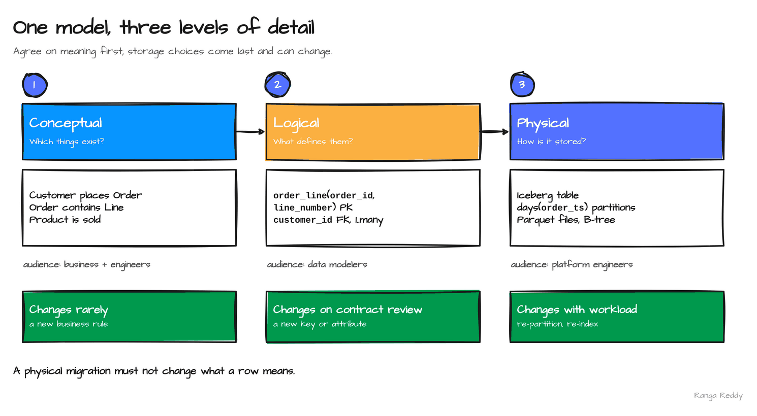
These levels answer different questions. Mixing them makes design reviews argue about implementation before agreeing on the business meaning.
Conceptual model
The conceptual model answers which business concepts exist and how they relate. Its artifact is an entity map or a domain model, drawn so a business owner can read it. In the sales example: customers place orders, orders contain lines, and products are sold.
Logical model
The logical model answers which attributes, keys, constraints, and cardinalities define the model. Its artifact is an ER model, a relational schema, or a dimensional model. In the sales example: one row per order line, with references to the customer, the product, and the date.
Physical model
The physical model answers how one specific engine stores and reads the model. Its artifacts are DDL, indexes, partitions, files, clustering, and distribution. In the sales example: PostgreSQL B-tree indexes, or Parquet files in an Iceberg table.
The same logical model can be implemented as PostgreSQL tables, Spark DataFrames, or Iceberg tables. The logical relationships should survive a storage migration. Physical choices can change when access patterns or engine capabilities change; a customer identifier is not a good physical partition key merely because it is an important logical key.
1.3 Core building blocks: entities, attributes, relationships, and constraints
In plain terms. Entities are the nouns (customer, product, order), attributes are their properties (email, price), relationships are the verbs (a customer places an order), and constraints are the rules (quantity must be positive).
An entity is a distinguishable business object or event, such as a customer, product, order, or payment. An attribute records a property of that entity. A relationship records how entities associate. A constraint states which values and combinations are valid.
For the order process, Customer and Product are entities; customer_id,
email, and country_code are attributes; Customer places Order is a
relationship. A constraint may state that an order-line quantity is positive
or that (order_id, line_number) is unique. A model should distinguish a
business fact from a convenient source-system column: a generated row number
does not become a durable product identity just because it is unique in one
extract.
The data type is part of the attribute contract. A monetary measure needs a
precision-preserving decimal and a currency policy; an event timestamp needs a
time-zone interpretation; an identifier that may contain leading zeroes is
usually text, not an integer. Types constrain values, but they do not capture
all business rules. Use NOT NULL, uniqueness, foreign keys, checks, and
pipeline assertions where the storage system can enforce them.
Four type mistakes come up again and again:
Postal codes stored as integers. postal_code = 02134 saved as an
integer becomes 2134, and the leading zero cannot be recovered. Store
postal codes as text.
Money stored as floating point. unit_price = 0.10 as a float or
double means 0.1 + 0.2 is not exactly 0.3, so totals drift by fractions
of a cent. Use DECIMAL(10, 2) with a separate currency column.
Timestamps without a time zone policy. An ordered_at value with no
declared zone reads as two different days in two regions. Store a timestamp
with a declared zone, such as UTC.
Flags stored as free text. An is_active column holding 'Y', 'N',
'yes' and NULL gives three spellings of one value, and filters miss rows.
Use a boolean with NOT NULL.
1.4 Identity management: primary keys, foreign keys, and alternate keys
In plain terms. A key is how you point at exactly one thing. Your passport number is a business key, issued by someone else. The seat number on your boarding pass is closer to a surrogate key, assigned by the airline for this one trip.
Primary key. Identifies one row in a relation. It is unique and non-null.
Example: (order_id, line_number) on an order line.
Foreign key. References a candidate key in another relation. Example:
fact_order_line.product_sk -> dim_product.product_sk.
Alternate key. A candidate identifier that was not chosen as the primary
key. Example: a unique email within a defined identity scope.
Business key. Identifies an entity in a source system or business
process. Example: customer_id issued by the CRM.
Surrogate key. A warehouse-controlled key for one model row or one
version of it. Example: customer_sk = 102 for one Type 2 version of a
customer.
Do not assume these mechanisms have equal enforcement in every platform. PostgreSQL constraints can reject a row that violates a primary key, foreign key, or unique constraint. Many lakehouse engines store table schemas and metadata without enforcing the same cross-table foreign-key contract during every write. In that case, the pipeline must test referential integrity explicitly.
Composite keys are not a modeling failure. They are often the honest source
identity, such as (order_id, line_number). Surrogate keys are useful when
source keys are unstable, multiple sources collide, or dimension history needs
a distinct key per version. A surrogate key generated independently on every
rebuild is not stable; preserve a key map or regenerate the facts that refer to
it.
Why both kinds exist. Two source systems can both use 1001 for different
customers, and one customer can have two versions of history. Neither problem
is solvable with the business key alone:
source   business key   meaning                 warehouse surrogate key
crm      1001           Ana Lopez               customer_sk = 101
billing  1001           Raj Kumar (collision)   customer_sk = 205
crm      1001           Ana Lopez, new segment  customer_sk = 102 (version 2)
1.5 Understanding cardinality and modality
In plain terms. Cardinality answers “how many?” and modality answers “is it required?” A customer can have zero or many orders; an order must have exactly one customer.
Cardinality describes how many instances can participate in a relationship. Modality (also called optionality or minimum cardinality) describes whether participation is optional or required. Read a relationship by its minimum and maximum on both ends:
Customer places Order. A customer has 0..many orders, and each order
has exactly 1 customer. A customer may have no orders yet, but no order
exists without a customer.
Order contains Line. An order has 1..many lines, and each line belongs
to exactly 1 order. A valid order has at least one line.
Product appears on Line. A product appears on 0..many lines, and each
line names exactly 1 product. A product may never have sold.
ER diagrams draw the same rule with crow’s-foot notation. The symbol nearest an entity describes how many of that entity participate:
  CUSTOMER ||--------o< ORDER ||--------|< ORDER_LINE >o--------|| PRODUCT

  ||   exactly one            o<   zero or many
  |<   one or many            >o   zero or many (drawn from the right)
Read the first link from left to right as “one customer places zero or many orders”, and from right to left as “each order belongs to exactly one customer”.
A many-to-many relationship usually needs an associative entity or bridge. For example, a sales line attributed to several campaigns cannot simply be joined to all campaigns and then summed: its amount is duplicated. Store the relationship at its own grain, then define whether queries filter through the bridge or allocate measures by weights. Section 2.2.2 runs that exact failure.
1.6 Types of data: structured, semi-structured, and unstructured
In plain terms. A spreadsheet is structured, a JSON API response is semi-structured, and a scanned invoice PDF is unstructured. The less structure the data has, the more of its model you must add yourself.
These terms describe how much organization is represented in the data, not whether it is important or valuable.
Structured data has named fields with stable types and relationships. Model it by declaring columns, keys, nullability, and meaning explicitly.
Semi-structured data is made of self-describing or nested records whose fields can vary, such as JSON events. Keep the source payload, project the governed fields into columns, and track schema versions.
Unstructured data has no stable row-and-column schema: documents, images, audio. Store the object itself, and model its searchable metadata, identity, ownership, and lifecycle separately.
JSON is not automatically a model, and Parquet is not automatically a good model. A nested payload may be the right raw representation for replay, while consumer-facing fields need explicit types, names, and evolution rules. A separate metadata row can model an image or document’s owner, classification, creation time, and object location without pretending its bytes are relational attributes.
Part 1 interview questions
1. What is data modeling, and why does a data engineer need it rather than just a DBA?
A data model is the agreed meaning of each dataset: what one row represents, which keys identify it, which time its attributes describe, and how its measures may be aggregated. Data engineers own the pipelines that create those rows, so they are the ones who either preserve that meaning or break it with a bad join, a blind append, or an untyped column. The DBA’s physical concerns, such as indexes and storage, come after the meaning is fixed.
2. Explain conceptual, logical, and physical models with one example.
Conceptual: “customers place orders, orders contain lines”. Logical:
order_line(order_id, line_number) is the primary key, customer_id is a
required foreign key, and a customer has zero or many orders. Physical: an
Iceberg table partitioned by days(order_ts), or a PostgreSQL table with a
B-tree index on customer_id. The strongest answer adds that the physical
level can change for performance without changing the logical meaning.
3. Business key vs surrogate key: why keep both?
The business key (customer_id = C01) identifies the real-world entity and is
how you match incoming source records. The surrogate key (customer_sk = 102)
is owned by the warehouse and identifies one row or one historical version.
You need the surrogate when sources collide on the same business key, when the
business key can change, or when Type 2 history needs a distinct key for each
version. Facts reference the surrogate so they point to the exact version that
was true at the event time.
4. What is the difference between cardinality and modality?
Cardinality is the maximum number of participants (one or many). Modality is
the minimum (zero means optional, one means mandatory). “A customer has 0..many
orders” is optional-many; “an order has exactly 1 customer” is
mandatory-one. Modality decides whether a foreign key can be NULL and
whether you need an “unknown” dimension member.
5. Why should money not be stored as a float?
Binary floating point cannot represent most decimal fractions exactly, so sums
of prices drift by small amounts and reconciliations fail. Use a fixed-point
DECIMAL(p, s) and store the currency alongside it. In Spark, multiplying two
decimals widens precision, so cast the result back to the declared contract
type, as the fact-table demo in section 3.5 does.
Part 2: Relational vs. Dimensional vs. Vault Modeling
2.1 Relational modeling: normalization (1NF-BCNF) vs. denormalization
In plain terms. Normalization means storing each fact in exactly one place. If a city name is written on every order, renaming the city means editing thousands of rows, and missing one leaves the data contradicting itself.
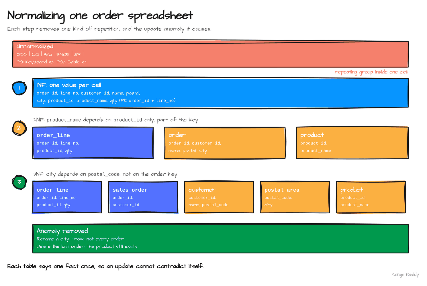
Normalization organizes a relational model to reduce update anomalies and inconsistent repetition. The normal forms are tests against a logical schema, not a contest to reach the largest possible number.
First normal form (1NF)
Each row-column position holds one value from the column’s domain, and
repeating groups become related rows. It prevents columns such as phone_1,
phone_2 and phone_3, which break the day a customer adds a fourth phone.
Second normal form (2NF)
The table is in 1NF, and every non-key attribute depends on the whole
candidate key, not on part of it. It prevents a product name repeated on
every (order_id, line_number) row when the name depends only on
product_id.
Third normal form (3NF)
The table is in 2NF, and no non-key attribute depends on the key through
another non-key attribute. It prevents customer_id -> postal_code -> city
from being stored redundantly on every order.
Boyce-Codd normal form (BCNF)
For every nontrivial functional dependency X -> Y, X is a superkey. It
catches determinants that are not candidate keys, which a schema can still
have while meeting 3NF.
The forms are stated with candidate keys and functional dependencies, not visual table aesthetics. BCNF is stricter than 3NF; decomposition can remove redundancy but may fail to preserve every dependency as a local constraint. Check whether the decomposed relations still enforce the business rules.
The three anomalies normalization removes. Each one is a way for the data to contradict itself:
Update anomaly. Renaming a city means editing every order row that
repeats it. After 3NF, the city lives in one postal_area row.
Insert anomaly. A new product cannot be stored until someone orders it.
After 3NF, you insert into product alone.
Delete anomaly. Deleting the only order for a product erases the product’s name. After 3NF, the product row exists independently of orders.
Run it. normalization.sql builds the 3NF schema from the diagram with
primary keys, foreign keys, and checks, then tries three bad inserts:
-- One fact per place: customers, products, orders and order lines in 3NF.
CREATE TABLE customer (
    customer_id   text PRIMARY KEY,
    email         text NOT NULL UNIQUE,
    postal_code   text NOT NULL
);

CREATE TABLE postal_area (
    postal_code   text PRIMARY KEY,
    city          text NOT NULL
);

ALTER TABLE customer
    ADD FOREIGN KEY (postal_code) REFERENCES postal_area (postal_code);

CREATE TABLE product (
    product_id    text PRIMARY KEY,
    product_name  text NOT NULL,
    list_price    numeric(10, 2) NOT NULL CHECK (list_price >= 0)
);

CREATE TABLE sales_order (
    order_id      text PRIMARY KEY,
    customer_id   text NOT NULL REFERENCES customer (customer_id),
    ordered_at    timestamptz NOT NULL
);

CREATE TABLE order_line (
    order_id      text NOT NULL REFERENCES sales_order (order_id),
    line_number   int  NOT NULL,
    product_id    text NOT NULL REFERENCES product (product_id),
    quantity      int  NOT NULL CHECK (quantity > 0),
    unit_price    numeric(10, 2) NOT NULL,
    PRIMARY KEY (order_id, line_number)
);

INSERT INTO postal_area VALUES ('94105', 'San Francisco'), ('10001', 'New York');
INSERT INTO customer VALUES ('C01', 'ana@example.com', '94105'),
                            ('C02', 'raj@example.com', '10001');
INSERT INTO product VALUES ('P01', 'Keyboard', 10.00), ('P02', 'Cable', 5.00);
INSERT INTO sales_order VALUES ('O1001', 'C01', '2025-01-15 10:00:00+00');
INSERT INTO order_line VALUES ('O1001', 1, 'P01', 2, 10.00),
                              ('O1001', 2, 'P02', 3, 5.00);

-- The constraints reject bad rows instead of storing them.
INSERT INTO order_line VALUES ('O1001', 3, 'P99', 1, 1.00);
INSERT INTO order_line VALUES ('O1001', 1, 'P02', 1, 5.00);
INSERT INTO order_line VALUES ('O1001', 4, 'P02', 0, 5.00);

-- A city rename touches one row, not every order.
UPDATE postal_area SET city = 'SF' WHERE postal_code = '94105';

SELECT o.order_id, l.line_number, c.customer_id, a.city,
       p.product_name, l.quantity * l.unit_price AS line_amount
FROM order_line l
JOIN sales_order o ON o.order_id = l.order_id
JOIN customer c    ON c.customer_id = o.customer_id
JOIN postal_area a ON a.postal_code = c.postal_code
JOIN product p     ON p.product_id = l.product_id
ORDER BY l.line_number;
PostgreSQL rejects each bad row with a named constraint, and the city rename updates one row:
ERROR:  insert or update on table "order_line" violates foreign key constraint "order_line_product_id_fkey"
DETAIL:  Key (product_id)=(P99) is not present in table "product".
ERROR:  duplicate key value violates unique constraint "order_line_pkey"
DETAIL:  Key (order_id, line_number)=(O1001, 1) already exists.
ERROR:  new row for relation "order_line" violates check constraint "order_line_quantity_check"
DETAIL:  Failing row contains (O1001, 4, P02, 0, 5.00).
UPDATE 1
 order_id | line_number | customer_id | city | product_name | line_amount
----------+-------------+-------------+------+--------------+-------------
 O1001    |           1 | C01         | SF   | Keyboard     |       20.00
 O1001    |           2 | C01         | SF   | Cable        |       15.00
The price of that safety is visible in the final query: four joins to reassemble one order line. That cost is what the next technique trades away.
Denormalization deliberately duplicates or precomputes information to serve a read workload. It trades simpler or faster reads for extra write, storage, and consistency obligations. A star schema denormalizes descriptive attributes into dimensions, while its fact table remains narrow and keyed. That is not the same as copying every source field into one enormous table.
| Normalized (3NF) | Denormalized (star, wide table) | |
|---|---|---|
| Optimized for | Many small, concurrent writes (OLTP) | Large scans and aggregations (OLAP) |
| Each fact stored | Once | Possibly many times |
| Joins per query | Many | Few |
| Risk | Slow analytical queries | Inconsistent copies if the load process is wrong |
2.2 Dimensional modeling core: fact tables vs. dimension tables
In plain terms. A fact table records things that happened and can be counted or summed: an order line with its quantity and amount. Dimension tables describe the who, what, where and when you filter and group by: customer, product, date. Questions such as “revenue by product category by month” read as facts sliced by dimensions.
Begin with a business event, not a target table. For sales, the source process might record an order with one or more product lines. A useful first statement is:
One row in
fact_order_linerepresents one product line accepted on one customer order.
That sentence is the grain declaration. It names the real-world measurement
event represented by one row. It is more useful than saying “the grain is
order_id, line_number”: those columns may implement the grain, but the
business sentence tells the team what the row means and which facts belong on
it. Kimball’s guidance is to declare the grain before selecting dimensions or
facts.
Once grain is clear, the design follows:
Operational events                 Analytical model
-------------------                 ----------------
orders + order lines  ----------->  fact_order_line
customer change log   ----------->  dim_customer (versioned)
product catalog       ----------->  dim_product
calendar              ----------->  dim_date

One accepted order line becomes one fact row.
Each dimension key identifies the entity version relevant to that line.
A fact table holds measurements of an event. Its columns are foreign keys
to dimensions plus numeric measures, so it is narrow and very long, and every
event adds a row. Example:
fact_order_line(order_date_key, customer_sk, product_sk, quantity, net_amount).
A dimension table holds descriptions of the things involved. Its columns
are a surrogate key, a business key, and many text attributes, so it is wide
and comparatively short. It grows only with new entities or new versions of
them. Example: dim_product(product_sk, product_id, name, category, brand).
The fact should contain measures that are true at this grain. For an order line, quantity, extended price, and line discount qualify. A customer lifetime total does not: it describes many orders and changes as more orders arrive. Store its derivation in the model or calculate it at query time, rather than repeating it on every line and making it additive by accident.
Grain controls joins as well as measures. If a dimension join matches two rows for one order line, the join has changed the fact grain. Every measure then appears twice. A model that passes a schema check can still be wrong by a factor of two; uniqueness and join-cardinality checks are correctness tests.
2.2.1 Choose the fact-table shape
The business process determines whether rows represent individual events, periodic states, or the progress of a workflow.
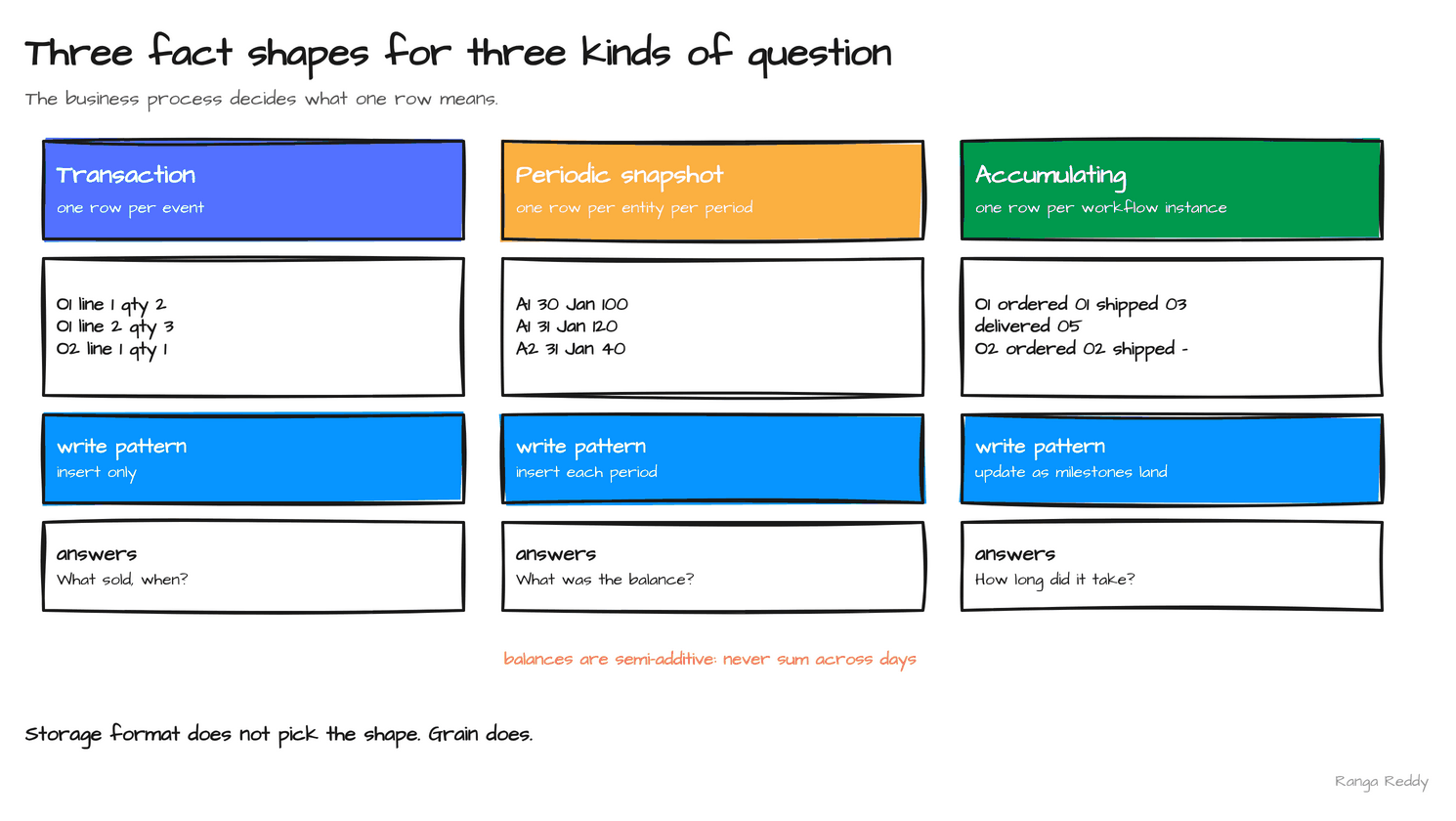
Transaction fact. One row is one event, such as an accepted order line. It gives the most flexible drill-down and reconciliation. The cost is a large, sparse, append-oriented table, where corrections need an explicit policy.
Periodic snapshot. One row is one entity at a regular interval, such as an account balance per day. It suits “as of” reporting and trend analysis. The table is predictably dense, and an unchanged balance is repeated every period.
Accumulating snapshot. One row is one workflow instance, updated as each milestone lands: order fulfilment, insurance claims, loan applications. It makes lifecycle analysis easy. The cost is that a row is revisited, and the earlier milestone values have to be managed.
These are modeling shapes, not storage formats. An Iceberg or Delta table can store any of them. A streaming pipeline can feed a transaction fact or update an accumulating snapshot; the table format does not decide what one row means.
A fourth shape is worth knowing for interviews: the factless fact, which
records that an event happened with no measure at all, such as a student
attending a class. Its only “measure” is COUNT(*).
2.2.2 Choose a serving model for its consumers
The staging model and the serving model need not have the same shape. Keep source-facing data faithful enough to replay and debug ingestion. Then publish a model whose joins, names, and measures match the questions consumers need to answer.
Normalized relational model. Use it for operational writes and consistent entity updates. Analytical queries pay for it with more joins and need shared semantic rules.
Dimensional star. Use it for BI filtering, grouping, and additive analysis. It requires a clear grain, conformed dimensions, and disciplined history handling.
Data Vault. Use it for auditable integration of several changing sources. It needs more structures and transformations before analysts find it comfortable.
One wide table. Use it for a narrow, stable workload or as a delivery boundary. It repeats attributes, makes history harder to express, and can multiply measures.
These patterns can coexist in layers. A raw CDC landing table is not a star schema, and a medallion label such as “silver” does not define a grain. Decide what contract each layer provides, then materialize the serving model for its actual workload.
Several dimension patterns change how a star model is queried without changing the fact grain:
- Conformed dimensions reuse the same definition and key domain across business processes, so sales and returns can be analyzed together.
- Role-playing dimensions use one logical dimension in multiple roles. An
order fact may carry
order_date_key,ship_date_key, anddelivery_date_key, all referencing the date dimension. - Degenerate dimensions keep a transaction identifier, such as
order_id, on the fact when a separate dimension would contain little more than that identifier. - Junk dimensions combine several low-cardinality flags, such as
is_gift,payment_typeandchannel, into one small dimension of their combinations, instead of adding many tiny dimensions or many flag columns to the fact. - Factless facts and bridge tables model events or many-to-many relationships without ordinary numeric measures. A bridge needs a filtering or allocation rule if joining it would repeat sales.
- Unknown and not-applicable members give missing references explicit keys. Do not collapse “not yet arrived,” “not collected,” “not applicable,” and “invalid source value” if they require different handling.
Classify each measure before publishing it:
Quantity sold is additive. It sums across order lines, products, and dates.
Net line amount is additive, with conditions. Sum it when each line appears once and currency is handled: within one currency, or after conversion to a declared reporting currency.
Unit price is non-additive. Recompute it as summed amount divided by summed quantity, or report a weighted measure. Never sum it.
Account balance is semi-additive. It sums across accounts but not across time. Pick a defined closing or as-of balance; never add daily balances together.
Margin percentage is a non-additive ratio. Recompute it from its additive numerator and denominator.
Never average a ratio by averaging row-level percentages unless the business definition explicitly requires an unweighted average. Retain the additive components needed to derive unit price, conversion rates, and percentages.
Run it. measures_demo.py puts the three classic measure traps side by
side: summing a semi-additive balance, averaging a ratio, and joining through
a bridge without weights.
"""Three measure traps: a semi-additive balance, a ratio, and a bridge table."""
from pyspark.sql import SparkSession

spark = (SparkSession.builder
         .appName("measures-demo")
         .config("spark.serializer", "org.apache.spark.serializer.KryoSerializer")
         .getOrCreate())

# A periodic snapshot: one row per account per day.
spark.createDataFrame([
    ("A1", "2025-01-30", 100.0), ("A1", "2025-01-31", 120.0),
    ("A2", "2025-01-30",  50.0), ("A2", "2025-01-31",  40.0),
], "account_id string, snapshot_date string, balance double") \
    .createOrReplaceTempView("fact_account_balance_daily")

wrong_balance = spark.sql(
    "SELECT sum(balance) FROM fact_account_balance_daily").first()[0]
closing_balance = spark.sql("""
    SELECT sum(balance) FROM fact_account_balance_daily
    WHERE snapshot_date = (SELECT max(snapshot_date) FROM fact_account_balance_daily)
""").first()[0]
print("sum of daily balances:", wrong_balance, "| closing balance:", closing_balance)
assert (wrong_balance, closing_balance) == (310.0, 160.0)

# Margin %: averaging row-level ratios weights a 10.00 sale like a 1,000.00 sale.
spark.createDataFrame([("L1", 1000.0, 100.0), ("L2", 10.0, 5.0)],
                      "line_id string, revenue double, margin double") \
    .createOrReplaceTempView("fact_sales")
avg_of_ratios, ratio_of_sums = spark.sql("""
    SELECT round(avg(margin / revenue) * 100, 2),
           round(sum(margin) / sum(revenue) * 100, 2)
    FROM fact_sales
""").first()
print("avg of row margins %:", avg_of_ratios, "| margin of totals %:", ratio_of_sums)
assert (avg_of_ratios, ratio_of_sums) == (30.0, 10.4)

# A bridge: order O1 is attributed to two campaigns with weights 0.7 and 0.3.
spark.createDataFrame([("O1", 200.0), ("O2", 50.0)],
                      "order_id string, net_amount double") \
    .createOrReplaceTempView("fact_order")
spark.createDataFrame([("O1", "EMAIL", 0.7), ("O1", "SEARCH", 0.3),
                       ("O2", "SEARCH", 1.0)],
                      "order_id string, campaign string, weight double") \
    .createOrReplaceTempView("bridge_order_campaign")

naive, allocated = spark.sql("""
    SELECT sum(f.net_amount), round(sum(f.net_amount * b.weight), 2)
    FROM fact_order f JOIN bridge_order_campaign b ON f.order_id = b.order_id
""").first()
print("revenue through bridge, naive:", naive, "| allocated:", allocated)
assert (naive, allocated) == (450.0, 250.0)

# The invariant that makes allocation safe: weights sum to 1 per order.
bad_weights = spark.sql("""
    SELECT count(*) FROM (SELECT order_id FROM bridge_order_campaign
                          GROUP BY order_id HAVING abs(sum(weight) - 1) > 1e-9)
""").first()[0]
assert bad_weights == 0

print("PASS: closing balance 160, margin 10.4%, allocated revenue 250")
spark.stop()
sum of daily balances: 310.0 | closing balance: 160.0
avg of row margins %: 30.0 | margin of totals %: 10.4
revenue through bridge, naive: 450.0 | allocated: 250.0
PASS: closing balance 160, margin 10.4%, allocated revenue 250
All three wrong answers come from valid SQL. Summing two days of balances
counts the same money twice. Averaging row margins lets a 10.00 sale weigh as
much as a 1,000.00 sale, giving 30% where the business margin is 10.4%. The
naive bridge join repeats order O1’s 200.00 once per campaign, reporting
450.00 of revenue for 250.00 of orders. The fix in each case is a modeling
rule, not a faster engine.
2.3 Schema topologies: star schema vs. snowflake schema
In plain terms. In a star schema the fact table sits in the middle and every dimension is one join away, like spokes on a wheel. A snowflake splits some dimensions into further tables (product, then subcategory, then category), so the drawing branches like a snowflake.
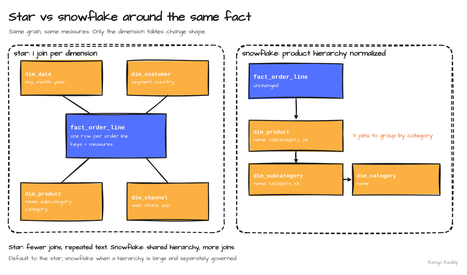
A star schema connects a fact directly to descriptive dimensions. A snowflake schema normalizes some dimension attributes into additional related tables. The difference is dimension topology, not fact grain.
Star. The typical form is
fact_sales -> dim_product(category, subcategory, ...). It gives fewer joins
and a compact semantic surface for common analysis. The cost is repeated
descriptions across product rows, so an attribute update touches more rows.
Snowflake. The typical form is
fact_sales -> dim_product -> dim_subcategory -> dim_category. Hierarchy
values are shared and dimension storage is less duplicated. The cost is more
joins, more relationship paths, and more chances for confusing filter
behavior.
Do not normalize a dimension merely because the source is normalized, and do not flatten every hierarchy automatically. Choose the form that makes the consumer contract understandable and can meet measured query and update requirements. A large, shared hierarchy with independently governed attributes may justify snowflaking; a small presentation dimension often benefits more from a direct star join.
A third topology, the galaxy or fact constellation, is several fact tables
sharing conformed dimensions: fact_order_line and fact_return_line both
join dim_product and dim_date, which is what makes “returns as a share of
sales by category” a valid query.
2.4 Data Vault 2.0: hubs, links, and satellites
In plain terms. Data Vault stores three things separately: the list of business keys that exist (hubs), which keys are connected (links), and every version of the descriptive details (satellites). Because each piece only ever grows, you can load from many sources at once and still audit exactly what arrived and when.
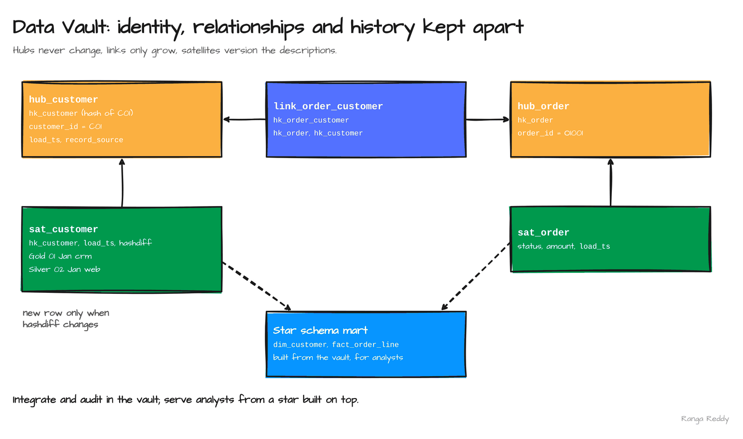
Data Vault separates durable business identity, relationships, and changing descriptions into different structures. A hub records a business key; a link records an association between hubs; a satellite records descriptive attributes and their history for a hub or link. Load time and source lineage are commonly retained so integrations can be audited.
This separation can help when multiple sources contribute changing records and the integration history must remain available. It also introduces more joins and more structures than most analysts should query directly. A common architecture uses a Vault as an integration/history layer and publishes star schemas as marts for reporting. Hash keys are a common implementation choice, not a substitute for canonicalizing business keys, testing collisions, or maintaining source identity.
Run it. data_vault_demo.py loads a hub and a satellite twice from two
sources. The same customer arrives as " c01 " and as "C01", and the second
load changes only one customer:
"""Load a Data Vault hub, link and satellite from two sources, twice.

Hash keys come from the canonicalized business key; the satellite only gains
a row when the hash of its descriptive attributes changes.
"""
from pyspark.sql import SparkSession, functions as F

spark = (SparkSession.builder
         .appName("data-vault-demo")
         .config("spark.serializer", "org.apache.spark.serializer.KryoSerializer")
         .config("spark.sql.session.timeZone", "UTC")
         .getOrCreate())


def hash_key(*cols):
    """SHA-256 over trimmed, upper-cased parts joined by a delimiter."""
    return F.sha2(F.concat_ws("||", *[F.upper(F.trim(F.col(c))) for c in cols]), 256)


def stage(df, source, load_ts):
    return (df
        .withColumn("hk_customer", hash_key("customer_id"))
        .withColumn("hashdiff", F.sha2(F.concat_ws("||",
                    F.coalesce(F.col("email"), F.lit("")),
                    F.coalesce(F.col("segment"), F.lit(""))), 256))
        .withColumn("record_source", F.lit(source))
        .withColumn("load_ts", F.to_timestamp(F.lit(load_ts))))


hub = spark.createDataFrame([], "hk_customer string, customer_id string, "
                                "record_source string, load_ts timestamp")
sat = spark.createDataFrame([], "hk_customer string, hashdiff string, email string, "
                                "segment string, record_source string, load_ts timestamp")


def load(hub, sat, staged):
    # Hub: insert business keys never seen before, from any source.
    new_keys = (staged
        .select("hk_customer", F.upper(F.trim("customer_id")).alias("customer_id"),
                "record_source", "load_ts")
        .dropDuplicates(["hk_customer"])
        .join(hub.select("hk_customer"), "hk_customer", "left_anti"))
    hub = hub.unionByName(new_keys)

    # Satellite: insert only when the latest stored hashdiff differs.
    latest = (sat.groupBy("hk_customer").agg(
        F.max_by("hashdiff", "load_ts").alias("last_hashdiff")))
    changed = (staged.join(latest, "hk_customer", "left")
        .filter(F.col("last_hashdiff").isNull()
                | (F.col("last_hashdiff") != F.col("hashdiff")))
        .select(sat.columns))
    return hub, sat.unionByName(changed)


crm_day1 = spark.createDataFrame(
    [(" c01 ", "ana@example.com", "Gold"), ("C02", "raj@example.com", "Silver")],
    "customer_id string, email string, segment string")
hub, sat = load(hub, sat, stage(crm_day1, "crm", "2025-01-01 02:00:00"))

# Day 2: C01 arrives again from the web shop in a different spelling and with
# a new segment; C02 is unchanged.
crm_day2 = spark.createDataFrame(
    [("C01", "ana@example.com", "Silver"), ("C02", "raj@example.com", "Silver")],
    "customer_id string, email string, segment string")
hub, sat = load(hub, sat, stage(crm_day2, "web", "2025-01-02 02:00:00"))

hub.select(F.substring("hk_customer", 1, 12).alias("hk_customer"),
           "customer_id", "record_source").orderBy("customer_id").show()
sat.select(F.substring("hk_customer", 1, 12).alias("hk_customer"),
           "segment", "record_source", F.col("load_ts").cast("date").alias("load_date")) \
   .orderBy("hk_customer", "load_ts").show()

assert hub.count() == 2           # " c01 " and "C01" are one customer
assert sat.count() == 3           # C01 twice, C02 once: no duplicate for C02

# A link records an association between hubs, here order -> customer.
orders = spark.createDataFrame([("O1001", "C01"), ("O1002", " c01")],
                               "order_id string, customer_id string")
link = (orders
    .withColumn("hk_order", hash_key("order_id"))
    .withColumn("hk_customer", hash_key("customer_id"))
    .withColumn("hk_order_customer", hash_key("order_id", "customer_id"))
    .select("hk_order_customer", "hk_order", "hk_customer"))
assert link.join(hub, "hk_customer").count() == 2

print("PASS: hub 2 keys, satellite 3 versions, link resolves to the hub")
spark.stop()
+------------+-----------+-------------+
| hk_customer|customer_id|record_source|
+------------+-----------+-------------+
|132bfbedb168|        C01|          crm|
|371e0b6ba48a|        C02|          crm|
+------------+-----------+-------------+

+------------+-------+-------------+----------+
| hk_customer|segment|record_source| load_date|
+------------+-------+-------------+----------+
|132bfbedb168|   Gold|          crm|2025-01-01|
|132bfbedb168| Silver|          web|2025-01-02|
|371e0b6ba48a| Silver|          crm|2025-01-01|
+------------+-------+-------------+----------+
PASS: hub 2 keys, satellite 3 versions, link resolves to the hub
Three behaviours to take from the output. Trimming and upper-casing before
hashing makes both spellings of C01 produce one hub row; skip that step and
the vault quietly holds two customers. The hub keeps the source that first
delivered the key, while each satellite row records its own source. And
C02, unchanged on day 2, gets no new satellite row, because its hashdiff
matched the latest stored one.
| Kimball star | Data Vault | 3NF (Inmon) warehouse | |
|---|---|---|---|
| Primary goal | Fast, understandable analysis | Auditable integration of many sources | One normalized enterprise model |
| History | SCD types on dimensions | Every satellite row, insert-only | Effective dates on entities |
| Loading | Transform, then load | Insert-only, highly parallel | Transform into the enterprise model |
| Query by analysts | Directly | Usually through marts | Usually through marts |
Part 2 interview questions
1. Explain 1NF, 2NF and 3NF with one example.
Start from an order row that lists several products in one cell. 1NF: one
value per cell, so each product becomes its own row keyed by
(order_id, line_number). 2NF: product_name depends only on product_id,
which is part of the key, so move it to a product table. 3NF: city
depends on postal_code, not on the key, so move it to a postal_area
table. Mention the anomaly each step removes: a city rename then updates one
row instead of every order.
2. When would you denormalize?
When the workload is read-heavy and join-heavy, as in analytics, and the duplicated attributes can be kept consistent by a controlled load process. A star schema is deliberate denormalization of dimensions. Do not denormalize a transactional system that takes many concurrent updates, because every copy becomes a place where the data can disagree.
3. What is grain, and why is it declared first?
Grain is what one row of a fact table represents, written as a business sentence: “one row per product line on an accepted order”. It is declared first because it decides which measures are valid on the row and which dimension joins are safe. A join that matches two rows per fact changes the grain and doubles every measure.
4. Additive, semi-additive, and non-additive measures: give an example of each.
Additive: quantity sold, which sums across every dimension. Semi-additive: account balance or inventory on hand, which sums across accounts but not across time; take the closing value per period instead. Non-additive: unit price or margin percentage; store the numerator and denominator and divide after summing. In the demo, averaging row margins gave 30% while the true margin was 10.4%.
5. Star vs snowflake: which would you choose?
Default to a star: fewer joins, simpler SQL for analysts, and BI tools handle it well. Snowflake a dimension when a hierarchy is large, shared by several dimensions, and governed separately, or when the storage saved by not repeating its values matters. The fact grain is the same either way.
6. What are conformed, role-playing, degenerate and junk dimensions?
Conformed: one dimension with the same keys and meaning, shared by several
facts, so sales and returns can be compared. Role-playing: one dimension used
in several roles, such as dim_date as order date, ship date and delivery
date. Degenerate: a transaction ID such as order_id kept on the fact with
no dimension table. Junk: one small dimension that holds the combinations of
several low-cardinality flags.
7. What are hubs, links and satellites, and why hash the business key?
A hub stores each unique business key once. A link stores a relationship
between hubs. A satellite stores descriptive attributes with load time and
source, and gets a new row only when the attributes change, detected by
comparing a hashdiff. Hashing the canonicalized business key gives a
deterministic key that any loader can compute independently, so hubs, links
and satellites load in parallel without looking up a sequence. Canonicalize
first: trim and upper-case, or " c01 " and "C01" become two customers.
8. How do you handle a many-to-many relationship between a fact and a dimension?
Use a bridge table at the grain of the relationship, such as
(order_id, campaign). Then either filter through it (“orders that touched
the EMAIL campaign”) without summing, or store allocation weights that sum to
1 per fact and multiply the measure by the weight. Test the sum-to-one
invariant. A plain join repeats the measure once per related row.
Part 3: Advanced Data Engineering Concepts & Storage Patterns
Part 2 defined the serving model. This part follows how that model changes as source data arrives, business attributes evolve, and storage formats change.
                         dim_date
                            |
dim_customer ---- fact_order_line ---- dim_product
                            |
                       dim_channel

fact_order_line grain: one row per order_id + line_number
Measures: quantity, gross_amount, discount_amount
3.1 Slowly Changing Dimensions (SCD Types 0–6 Deep Dive)
In plain terms. Customers move, products get renamed, sales reps change territory. An SCD type is the rule for what happens to history when a dimension attribute changes: forget the old value, keep it in a new row, or keep it in an extra column.
The SCD number is a response policy for changed attributes, not a property of the whole dimension table. Apply policies at the attribute level. Type 2 is the workhorse when historical facts must retain the dimension values that were true when the event occurred; other types fit distinct questions.
This guide follows Kimball’s named patterns. Type numbers beyond 1–3 are not used consistently by every vendor or author, so document the chosen behavior instead of relying on a number alone.
Type 0: retain the original
The first accepted value never changes. Use it when the original value is
durable by definition, or explicitly labeled “original”, such as
original_signup_channel.
Type 1: overwrite
Only the latest value is kept. Use it to correct an error, or when the business intentionally restates all history with the new value.
Type 2: add a row
Each effective version gets its own row and its own surrogate key. Use it when historical facts must resolve to the attribute version that was valid at event time. This is the type interviews ask about most.
Type 3: add a column
The row keeps the current value plus one or a few prior values in extra columns. Use it when a limited comparison, such as current region versus previous region, is enough.
Type 4: mini-dimension
Volatile attributes move to a separate dimension of attribute profiles. Use it when several attributes change rapidly, or their combinations would explode the base dimension.
Type 5: mini-dimension plus a current pointer
Type 4 profile history, plus a Type 1 reference to the current profile on the base dimension. Use it when facts need the historical profile and consumers also want easy access to the current one.
Type 6: hybrid of Types 1, 2 and 3
Version rows, plus current-value columns overwritten on every historical row. Use it when consumers need both “as was” and “as is” reporting without a separate current-key join.
The same change under four types. Customer C01 moves from Gold to
Silver on 1 February. This is what dim_customer holds afterwards:
Type 0  (keep original)
  customer_sk  customer_id  segment
  101          C01          Gold        <- the change is ignored

Type 1  (overwrite)
  customer_sk  customer_id  segment
  101          C01          Silver      <- January sales now report as Silver

Type 2  (new row)
  customer_sk  customer_id  segment  valid_from  valid_to    is_current
  101          C01          Gold     2025-01-01  2025-02-01  false
  102          C01          Silver   2025-02-01  9999-12-31  true

Type 3  (new column)
  customer_sk  customer_id  segment  previous_segment
  101          C01          Silver   Gold                <- one step of history
Types 5 and 6 duplicate or update information to make current-state questions easier. That convenience creates maintenance work: every affected Type 6 version row must receive the current overlay, and a Type 5 current pointer must be updated when the profile changes. If that synchronization is late, “current” attributes become stale while the Type 2 history may still be correct.
Keep business identity separate from warehouse identity
A business key comes from the source domain: customer_id = C01 identifies
the customer across source updates. A surrogate key is assigned by the
warehouse to identify one dimension row or version, for example
customer_sk = 101 for the customer’s Gold version and customer_sk = 102
for the later Silver version.
The fact normally stores the surrogate key. If the customer changes segment,
the current source key remains C01, but the new dimension version receives a
new surrogate key. This preserves both identity and history. A generated
surrogate key must be stable across incremental runs; monotonically_increasing_id()
and an unpersisted row_number() are not durable key-assignment strategies.
Use a persisted key map or the warehouse platform’s governed key-generation
process.
Composite business keys are valid when they describe source identity. If a
source identifies an order line with (order_id, line_number), do not discard
one part and hope the remaining ID is unique. Preserve the components or map
them to a stable key, and test uniqueness at the declared grain.
Type 2: make dimension history explicit
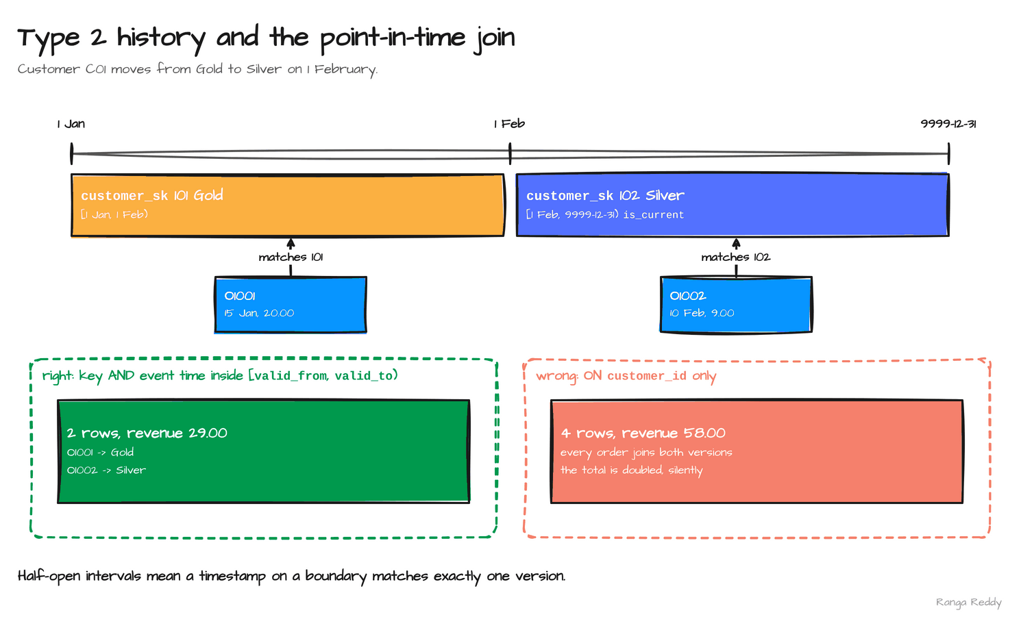
For Type 2, model a half-open validity interval [valid_from, valid_to). The
old version is valid at its start and stops being valid exactly when the next
version starts. Half-open intervals avoid double matches at a boundary:
customer_id  customer_sk  segment  valid_from           valid_to
C01          101          Gold     2025-01-01 00:00:00  2025-02-01 00:00:00
C01          102          Silver   2025-02-01 00:00:00  9999-12-31 00:00:00
To attach the right customer to a sale, match both the business key and event time:
o.customer_id = c.customer_id
AND o.order_ts >= c.valid_from
AND o.order_ts <  c.valid_to
Joining on customer_id alone can match every historical version and multiply
the sale. Joining only to the current row keeps one result but restates old
sales using today’s attributes. Neither is a harmless implementation choice;
they answer different business questions.
Run it: SCD Type 1 and Type 2 with Iceberg MERGE. A Type 2 load has to do
two things for each changed customer in one atomic step: close the current
version and insert the new one. A single MERGE can only take one action per
source row, so the standard trick stages each changed customer twice. One
copy carries the real key and matches the current version, which gets closed.
The other copy carries a NULL merge key, matches nothing, and is inserted as
the new version. scd_merge_demo.py does that, then applies a Type 1
overwrite of email across all versions, then runs the point-in-time join:
"""SCD Type 1 and Type 2 on an Iceberg dimension, then a point-in-time fact join.

Runs on datalake-playground's spark-master in local mode. The Iceberg catalog
is a Hadoop catalog on the container's local disk, so nothing touches the
shared metastore or MinIO.
"""
from pyspark.sql import SparkSession

spark = (SparkSession.builder
         .appName("scd-merge-demo")
         .config("spark.sql.extensions",
                 "org.apache.iceberg.spark.extensions.IcebergSparkSessionExtensions")
         .config("spark.serializer", "org.apache.spark.serializer.KryoSerializer")
         .config("spark.sql.catalog.dm", "org.apache.iceberg.spark.SparkCatalog")
         .config("spark.sql.catalog.dm.type", "hadoop")
         .config("spark.sql.catalog.dm.warehouse", "file:///tmp/dm_blog/warehouse")
         .config("spark.sql.session.timeZone", "UTC")
         .getOrCreate())

spark.sql("CREATE NAMESPACE IF NOT EXISTS dm.sales")
spark.sql("DROP TABLE IF EXISTS dm.sales.dim_customer PURGE")
spark.sql("""
    CREATE TABLE dm.sales.dim_customer (
        customer_sk  BIGINT    NOT NULL,
        customer_id  STRING    NOT NULL,
        email        STRING,
        segment      STRING,
        valid_from   TIMESTAMP NOT NULL,
        valid_to     TIMESTAMP NOT NULL,
        is_current   BOOLEAN   NOT NULL
    ) USING iceberg
""")

# Initial load: three customers, all valid from 1 January.
spark.sql("""
    INSERT INTO dm.sales.dim_customer VALUES
    (101, 'C01', 'ana@example.com',  'Gold',   TIMESTAMP '2025-01-01', TIMESTAMP '9999-12-31', true),
    (201, 'C02', 'raj@example.com',  'Silver', TIMESTAMP '2025-01-01', TIMESTAMP '9999-12-31', true),
    (301, 'C03', 'li@example.com',   'Bronze', TIMESTAMP '2025-01-01', TIMESTAMP '9999-12-31', true)
""")

# The 1 February batch: C01 changes segment (Type 2), C02 changes only its
# email (Type 1), C03 is unchanged, and C04 is new.
spark.createDataFrame(
    [("C01", "ana@example.com",     "Silver", "2025-02-01 00:00:00"),
     ("C02", "raj.k@example.com",   "Silver", "2025-02-01 00:00:00"),
     ("C03", "li@example.com",      "Bronze", "2025-02-01 00:00:00"),
     ("C04", "sam@example.com",     "Gold",   "2025-02-01 00:00:00")],
    "customer_id string, email string, segment string, effective_from string",
).selectExpr("*", "CAST(effective_from AS TIMESTAMP) AS effective_ts") \
 .createOrReplaceTempView("customer_updates")

# New surrogate keys come from the table's current maximum, so a key, once
# written, never changes on a later run.
spark.sql("""
    CREATE OR REPLACE TEMP VIEW staged AS
    WITH changed AS (
        SELECT u.*
        FROM customer_updates u
        LEFT JOIN dm.sales.dim_customer d
          ON d.customer_id = u.customer_id AND d.is_current
        WHERE d.customer_id IS NULL OR d.segment <> u.segment
    ),
    keyed AS (
        SELECT c.*,
               (SELECT max(customer_sk) FROM dm.sales.dim_customer)
               + row_number() OVER (ORDER BY c.customer_id) AS new_sk
        FROM changed c
    )
    -- Row 1 per change: matches the current version and closes it.
    SELECT customer_id AS merge_key, * FROM keyed
    UNION ALL
    -- Row 2 per change: matches nothing, so it inserts the new version.
    SELECT NULL AS merge_key, * FROM keyed
""")

# Type 2: close the old version and open a new one.
spark.sql("""
    MERGE INTO dm.sales.dim_customer t
    USING staged s
    ON t.customer_id = s.merge_key AND t.is_current
    WHEN MATCHED THEN UPDATE SET
        t.valid_to   = s.effective_ts,
        t.is_current = false
    WHEN NOT MATCHED AND s.merge_key IS NULL THEN INSERT
        (customer_sk, customer_id, email, segment, valid_from, valid_to, is_current)
        VALUES (s.new_sk, s.customer_id, s.email, s.segment,
                s.effective_ts, TIMESTAMP '9999-12-31', true)
""")

# Type 1: overwrite email on every version of the customer, history included.
spark.sql("""
    MERGE INTO dm.sales.dim_customer t
    USING customer_updates u
    ON t.customer_id = u.customer_id
    WHEN MATCHED AND t.email <> u.email THEN UPDATE SET t.email = u.email
""")

dim = spark.sql("""
    SELECT customer_sk, customer_id, email, segment,
           CAST(valid_from AS DATE) AS valid_from,
           CAST(valid_to AS DATE)   AS valid_to, is_current
    FROM dm.sales.dim_customer ORDER BY customer_id, valid_from
""")
dim.show(truncate=False)

rows = {r.customer_sk: r for r in dim.collect()}
assert len(rows) == 5
assert not rows[101].is_current and str(rows[101].valid_to) == "2025-02-01"
assert rows[302].customer_id == "C01" and rows[302].segment == "Silver"
assert rows[303].customer_id == "C04"
assert rows[201].email == "raj.k@example.com" and rows[201].is_current

# Validity intervals for one customer never overlap.
overlaps = spark.sql("""
    SELECT count(*) FROM dm.sales.dim_customer a
    JOIN dm.sales.dim_customer b
      ON a.customer_id = b.customer_id AND a.customer_sk < b.customer_sk
     AND a.valid_from < b.valid_to AND b.valid_from < a.valid_to
""").first()[0]
assert overlaps == 0

# Point-in-time join: each order picks the version valid when it happened.
spark.createDataFrame(
    [("O1001", "C01", "2025-01-15 10:00:00", 20.00),
     ("O1002", "C01", "2025-02-10 11:00:00",  9.00)],
    "order_id string, customer_id string, ordered_at string, net_amount double",
).selectExpr("*", "CAST(ordered_at AS TIMESTAMP) AS order_ts") \
 .createOrReplaceTempView("orders")

point_in_time = spark.sql("""
    SELECT o.order_id, d.customer_sk, d.segment AS segment_at_order, o.net_amount
    FROM orders o
    JOIN dm.sales.dim_customer d
      ON o.customer_id = d.customer_id
     AND o.order_ts >= d.valid_from AND o.order_ts < d.valid_to
    ORDER BY o.order_id
""")
point_in_time.show()
assert [r.segment_at_order for r in point_in_time.collect()] == ["Gold", "Silver"]

# The tempting join on customer_id alone doubles every C01 order.
wrong = spark.sql("""
    SELECT count(*) AS joined_rows, sum(o.net_amount) AS revenue
    FROM orders o JOIN dm.sales.dim_customer d ON o.customer_id = d.customer_id
""").first()
print("customer_id-only join:", wrong.joined_rows, "rows, revenue", wrong.revenue)
assert wrong.joined_rows == 4 and wrong.revenue == 58.0

spark.sql("SELECT operation "
          "FROM dm.sales.dim_customer.snapshots ORDER BY committed_at").show()
print("PASS: 5 customer versions, no overlaps, point-in-time join correct")
spark.stop()
+-----------+-----------+-----------------+-------+----------+----------+----------+
|customer_sk|customer_id|email            |segment|valid_from|valid_to  |is_current|
+-----------+-----------+-----------------+-------+----------+----------+----------+
|101        |C01        |ana@example.com  |Gold   |2025-01-01|2025-02-01|false     |
|302        |C01        |ana@example.com  |Silver |2025-02-01|9999-12-31|true      |
|201        |C02        |raj.k@example.com|Silver |2025-01-01|9999-12-31|true      |
|301        |C03        |li@example.com   |Bronze |2025-01-01|9999-12-31|true      |
|303        |C04        |sam@example.com  |Gold   |2025-02-01|9999-12-31|true      |
+-----------+-----------+-----------------+-------+----------+----------+----------+

+--------+-----------+----------------+----------+
|order_id|customer_sk|segment_at_order|net_amount|
+--------+-----------+----------------+----------+
|   O1001|        101|            Gold|      20.0|
|   O1002|        302|          Silver|       9.0|
+--------+-----------+----------------+----------+

customer_id-only join: 4 rows, revenue 58.0
+---------+
|operation|
+---------+
|   append|
|overwrite|
|overwrite|
+---------+
PASS: 5 customer versions, no overlaps, point-in-time join correct
Read the result row by row. C01 changed segment, so version 101 was
closed at 1 February and version 302 opened. C02 changed only its email,
a Type 1 attribute, so it was overwritten in place with no new version. C03
was unchanged and untouched. C04 was new and got its first version. New
surrogate keys continue from the table’s maximum (301), so keys already
written never change on a rerun. Each MERGE committed as one Iceberg
snapshot (overwrite), so a reader never sees a closed version without its
replacement.
The final check is the one that matters for reports: the point-in-time join
returns two rows and 29.00, while the customer_id-only join returns four rows
and 58.00 with no error.
3.2 Change Data Capture (CDC): mechanics and design patterns
In plain terms. Instead of copying a whole table every night, CDC reads the database’s own change journal and ships only what changed: this row was inserted, that one updated, this one deleted. The hard part is not capturing the changes; it is applying them in the right order, exactly once in effect.
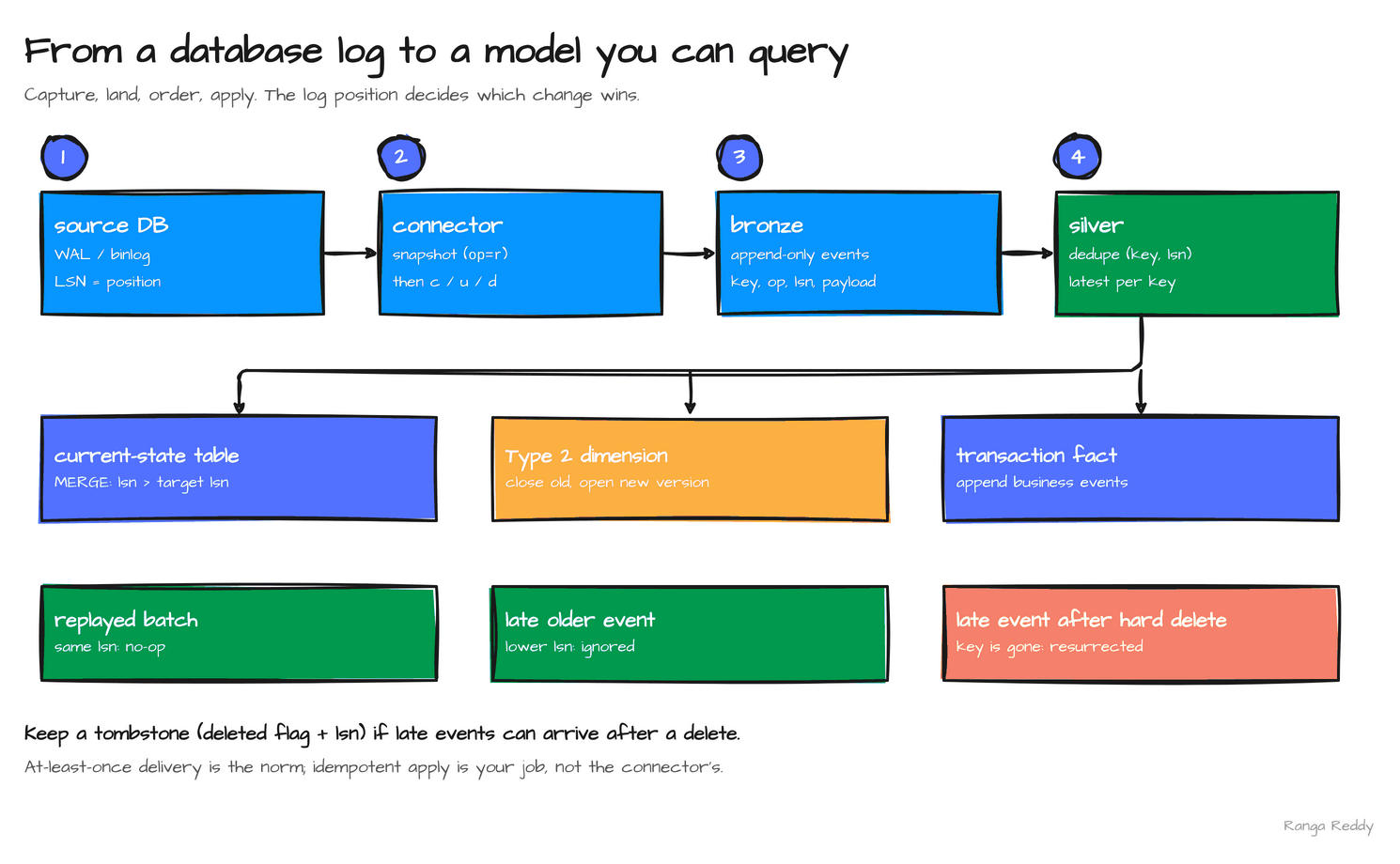
Change Data Capture records changes at the source boundary so downstream systems can maintain a copy without repeatedly scanning the entire source. There are three common capture paths:
Log-based CDC reads the database transaction log or WAL. The operational concerns are log retention, replication slots, privileges, and source-specific ordering.
Trigger-based CDC reads changes that database triggers write to an outbox or audit table. The concerns are trigger overhead, transaction behavior, and cleanup of the capture table.
Query-based CDC polls periodically with a timestamp or a monotonically increasing key. Deletes and intermediate updates can be invisible, and timestamps can arrive late or be non-unique.
Log-based CDC is not simply “a stream of row JSON.” A Debezium event can include a key, before/after values, operation type, source metadata and log position. A connector may first emit a consistent snapshot, then continue from the corresponding log position. Consumers must distinguish snapshot reads from inserts, updates, deletes, and tombstones, and must use the source’s ordering metadata rather than a connector processing timestamp when ordering matters.
Source transaction log
        |
        v
CDC connector: snapshot + ordered change events
        |
        v
Immutable landing log: key, op, source position, event time, payload
        |
        v
Deduplicate and order -> current-state tables / SCDs / facts
The raw event log and the analytical model answer different questions. The event log is useful for replay and audit. A current-state table applies the latest accepted operation per key. A Type 2 dimension turns selected attribute changes into effective versions. A transaction fact records business events at their declared grain. Do not interpret every update as a new business event, or every delete as a physical row removal.
Define how the consumer handles at-least-once delivery: retain a source position such as an LSN or log offset, use a stable row key and deterministic ordering, make replays idempotent, and test duplicate delivery. A primary-key change may be represented as deletion of the old key plus insertion of the new key. A source snapshot can also overlap the live stream unless the connector’s snapshot protocol resolves that boundary. The pipeline’s idempotency and ordering rules must cover both cases.
CDC application patterns
- Append-only event fact: keep each distinct business event and deduplicate by event identity. Preserve correction events instead of silently rewriting a prior event when the business requires an audit trail.
- Current-state upsert: group changes by business key and apply them in source order. A delete becomes a tombstone or explicit deleted state if downstream consumers need to know that the key existed.
- Type 2 history: compare tracked attributes, expire the current version, and insert a new version with effective-time boundaries.
- Snapshot plus stream: bootstrap from a consistent snapshot and continue from its source-log boundary. Reconciliation compares the snapshot’s key set and values with the resulting target state.
CDC does not provide free exactly-once business effects. A sink may commit a row while the offset commit fails, causing a replay. Coordinate the sink transaction and offset where supported; otherwise use idempotent writes and durable source positions.
Run it: apply CDC idempotently. cdc_apply_demo.py takes seven
Debezium-style events for three customers, including a snapshot, two updates
to one key, a delete, an insert, and one redelivered event. It then replays
the batch, sends a late older event, and finally shows the trap that hard
deletes create:
"""Apply a batch of Debezium-style change events to an Iceberg current-state table.

The batch contains a snapshot, two updates to one key, a delete, an insert and
a redelivered event. Applying it twice must leave the table unchanged.
"""
from pyspark.sql import SparkSession, Window, functions as F

spark = (SparkSession.builder
         .appName("cdc-apply-demo")
         .config("spark.sql.extensions",
                 "org.apache.iceberg.spark.extensions.IcebergSparkSessionExtensions")
         .config("spark.serializer", "org.apache.spark.serializer.KryoSerializer")
         .config("spark.sql.catalog.dm", "org.apache.iceberg.spark.SparkCatalog")
         .config("spark.sql.catalog.dm.type", "hadoop")
         .config("spark.sql.catalog.dm.warehouse", "file:///tmp/dm_blog/warehouse")
         .config("spark.sql.session.timeZone", "UTC")
         .getOrCreate())

spark.sql("CREATE NAMESPACE IF NOT EXISTS dm.sales")
spark.sql("DROP TABLE IF EXISTS dm.sales.customer_current PURGE")
spark.sql("""
    CREATE TABLE dm.sales.customer_current (
        customer_id  STRING NOT NULL,
        email        STRING,
        segment      STRING,
        source_lsn   BIGINT NOT NULL
    ) USING iceberg
""")

# op: r = snapshot read, c = create, u = update, d = delete.
# lsn is the source log position; it, not arrival order, decides which wins.
events = spark.createDataFrame([
    ("r",  1, "C01", "ana@example.com",   "Gold"),
    ("r",  2, "C02", "raj@example.com",   "Silver"),
    ("u", 10, "C01", "ana@example.com",   "Silver"),
    ("d", 11, "C02", None,                None),
    ("u", 12, "C01", "ana.m@example.com", "Silver"),
    ("c", 13, "C05", "kim@example.com",   "Bronze"),
    ("u", 12, "C01", "ana.m@example.com", "Silver"),   # redelivered
], "op string, lsn bigint, customer_id string, email string, segment string")

# Keep the latest event per key. Exact redeliveries collapse first.
latest = (events
    .dropDuplicates(["customer_id", "lsn"])
    .withColumn("rn", F.row_number().over(
        Window.partitionBy("customer_id").orderBy(F.col("lsn").desc())))
    .filter("rn = 1")
    .drop("rn"))
latest.orderBy("customer_id").show()
latest.createOrReplaceTempView("latest_changes")

apply_sql = """
    MERGE INTO dm.sales.customer_current t
    USING latest_changes s
    ON t.customer_id = s.customer_id
    WHEN MATCHED AND s.op = 'd' AND s.lsn > t.source_lsn THEN DELETE
    WHEN MATCHED AND s.op <> 'd' AND s.lsn > t.source_lsn THEN UPDATE SET
        t.email = s.email, t.segment = s.segment, t.source_lsn = s.lsn
    WHEN NOT MATCHED AND s.op <> 'd' THEN INSERT
        (customer_id, email, segment, source_lsn)
        VALUES (s.customer_id, s.email, s.segment, s.lsn)
"""
spark.sql(apply_sql)
first = spark.table("dm.sales.customer_current").orderBy("customer_id")
first.show()
first_rows = [tuple(r) for r in first.collect()]
assert first_rows == [("C01", "ana.m@example.com", "Silver", 12),
                      ("C05", "kim@example.com", "Bronze", 13)]

# Replay the same batch, as an at-least-once consumer will after a crash.
spark.sql(apply_sql)
replayed = [tuple(r) for r in
            spark.table("dm.sales.customer_current").orderBy("customer_id").collect()]
assert replayed == first_rows

# An older event arriving late must not overwrite a newer one.
spark.createDataFrame([("u", 10, "C01", "ana@example.com", "Silver")],
                      events.schema).createOrReplaceTempView("latest_changes")
spark.sql(apply_sql)
assert spark.table("dm.sales.customer_current") \
            .filter("customer_id = 'C01'").first().source_lsn == 12

# The trap: C02 was hard-deleted, so the target no longer remembers lsn 11.
# A late update older than the delete now looks like a brand-new key.
spark.createDataFrame([("u", 2, "C02", "raj@example.com", "Silver")],
                      events.schema).createOrReplaceTempView("latest_changes")
spark.sql(apply_sql)
resurrected = spark.table("dm.sales.customer_current") \
                   .filter("customer_id = 'C02'").count()
print("C02 rows after a late pre-delete event:", resurrected)
assert resurrected == 1

print("PASS: 7 events -> 2 rows; replay and late update were no-ops; "
      "late event after a hard delete resurrected C02")
spark.stop()
+---+---+-----------+-----------------+-------+
| op|lsn|customer_id|            email|segment|
+---+---+-----------+-----------------+-------+
|  u| 12|        C01|ana.m@example.com| Silver|
|  d| 11|        C02|             NULL|   NULL|
|  c| 13|        C05|  kim@example.com| Bronze|
+---+---+-----------+-----------------+-------+

+-----------+-----------------+-------+----------+
|customer_id|            email|segment|source_lsn|
+-----------+-----------------+-------+----------+
|        C01|ana.m@example.com| Silver|        12|
|        C05|  kim@example.com| Bronze|        13|
+-----------+-----------------+-------+----------+
C02 rows after a late pre-delete event: 1
PASS: 7 events -> 2 rows; replay and late update were no-ops; late event after a hard delete resurrected C02
Three guards make the apply idempotent. Exact redeliveries collapse on
(customer_id, lsn). Only the highest lsn per key survives, so the
intermediate update at lsn = 10 is never written. Every MATCHED branch
requires s.lsn > t.source_lsn, so a replay or an older straggler changes
nothing.
The last step shows what those guards cannot protect. Once C02 is
physically deleted, the target has no row left to remember that lsn = 11
was its last change. A late event at lsn = 2 arrives, hits NOT MATCHED,
and inserts the customer again. If late or out-of-order delivery is possible,
keep a tombstone (is_deleted = true plus the delete’s lsn) instead of
removing the row, and purge tombstones only after the maximum lateness window
has passed.
3.3 Storage evolution: warehouses vs. data lakes vs. data lakehouses
In plain terms. A warehouse is a managed database tuned for SQL analytics. A lake is cheap file storage that holds anything. A lakehouse adds a table format such as Iceberg on top of the lake’s files, so many engines can share tables with transactions, schemas, and snapshots.
These names describe broad storage and access patterns, not one required product or modeling method.
Data warehouse. It provides managed SQL tables, transaction processing, catalogs, and query optimization. Curated schemas and constraints sit close to the serving engine. What it does not give you by itself is agreement on metric meaning or source history.
Data lake. It provides low-cost files and object storage for varied data and compute engines. Raw, semi-structured, and curated data can coexist, so contracts need explicit owners. Storing Parquet files does not give you atomic table transactions.
Data lakehouse. It provides lake storage plus an open table format and a metadata and catalog layer. Several engines can share schemas, snapshots, and table-level commits. It still does not give you every relational constraint, cross-table transactions, or semantic definitions.
Parquet is a file format. Iceberg, Delta Lake, and Hudi add table metadata and commit behavior around data files; they do not make the data model correct. Table-level atomicity is also not automatically a transaction spanning several tables. If a fact and dimension publish in separate commits, define how consumers identify a compatible model version or batch.
Medallion architecture: bronze, silver, and gold
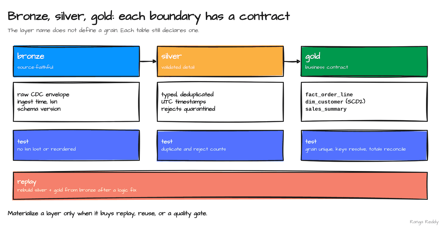
Medallion architecture is a way to organize a lakehouse’s data lifecycle into progressively more validated and purpose-shaped layers. It is a logical pattern, not a different fact-table design, a particular file format, or a requirement that every transformation create another physical table. The bronze/silver/gold labels also do not define row grain; each table still needs its own contract.
Bronze preserves the source. It keeps source-shaped records and ingestion metadata for replay and audit. In the sales example, that is the raw order CDC envelope with key, operation, source position, and before/after payload. Keep source identity, capture time, source event time, and schema version explicit.
Silver cleans the detail. It validates, types, deduplicates, and standardizes detailed records: curated order lines and customer change history with normalized timestamps and currencies. Keep business keys, source ordering, invalid-row handling, and Type 2 effective-time rules explicit.
Gold publishes the contract. It holds business-facing dimensional models
and workload-specific aggregates: fact_order_line, dim_customer,
dim_product, and sales summaries. Keep the declared grain, conformed
dimensions, measure definitions, freshness, and consumer contract explicit.
CDC snapshot + change log
     |
     v
   bronze.order_events       source-faithful, replayable
     |
     v
   silver.order_line         validated grain and types
   silver.customer_change    ordered source history
     |
     v
   gold.fact_order_line      one row per order line
   gold.dim_customer         governed customer versions
   gold.sales_summary        measures defined for reporting
For the running example, Bronze retains the original event envelope so a parser or business-rule change can be replayed. Silver resolves duplicate delivery using the source key and log position, applies delete semantics, and quarantines malformed rows instead of silently dropping them. Gold performs the Type 2 lookup using the order’s event time and publishes the tested order-line fact. A gold layer can contain detailed facts as well as aggregates; “gold means aggregated” is a convention, not a data-model rule.
Do not force every intermediate DataFrame into a permanent layer. Materialize a boundary when it supports replay, independent reuse, quality enforcement, ownership, or a measured workload. Otherwise, extra tables add storage, commits, metadata, orchestration, and schema contracts without adding a useful recovery point. The layering pattern is recommended in some lakehouse platforms, but it is not mandatory; choose boundaries that fit the system’s failure and consumption requirements.
Test each transition independently. Bronze-to-silver should prove source positions are neither lost nor applied out of order. Silver should expose duplicate and rejected-row counts. Gold should prove fact grain, dimension coverage, Type 2 non-overlap, and reconciled measures. A single end-to-end row count cannot identify which boundary lost or multiplied records.
3.4 Schema evolution and data contracts
In plain terms. A data contract is the promise a producer makes to its consumers: these columns, with these types and meanings, changed only by these rules. Schema evolution is how a table changes shape without breaking the people who read it.
A schema contract is more than a list of field names. It should state field types, nullability, meaning, units, valid values, key semantics, event-time meaning, privacy classification, and compatibility expectations. Version the contract and identify an owner who can approve changes.
Adding a nullable field is often compatible, depending on the consumer. Ask what null means for old rows, and which contract version adds the field.
Renaming a field is not automatically compatible. Ask whether it is the same semantic field or a new definition, and provide a migration alias or a transition period.
Widening a numeric type is often compatible if values keep their meaning. Ask whether the target engine supports the widening, and whether every producer can write it.
Narrowing or reinterpreting a type is usually breaking. Plan the backfill, the validation, and the consumer migration.
Changing a metric definition is semantically breaking even when the SQL type does not change. Version the metric or publish a new one, because schema compatibility cannot preserve meaning.
Parquet readers may infer different schemas from different files. Spark supports schema merging, but it is disabled by default because collecting schemas across files has a cost. For table formats, schema and partition evolution are metadata operations with format-specific compatibility rules. Validate the logical contract before accepting either change.
A contract can be as small as a reviewed YAML file next to the pipeline code. What matters is that each line is something a test can check:
dataset: gold.fact_order_line
owner: sales-data-team
version: 2
grain: one row per product line on an accepted customer order
primary_key: [order_id, line_number]
columns:
  - {name: order_id,       type: string,        nullable: false}
  - {name: line_number,    type: int,           nullable: false}
  - {name: order_date_key, type: int,           nullable: false}
  - {name: customer_sk,    type: int,           nullable: false, references: dim_customer.customer_sk, unknown_member: -1}
  - {name: product_sk,     type: int,           nullable: false, references: dim_product.product_sk,   unknown_member: -1}
  - {name: net_amount,     type: decimal(12,2), nullable: false, rule: gross_amount - discount_amount, currency: USD}
compatibility: backward       # add nullable columns only; renames need a new version
freshness: loaded by 06:00 UTC daily
3.5 Hands-on: build the fact table end to end
The example starts with curated order lines and customer change records. It derives end-exclusive customer validity ranges, resolves the customer version at order time, joins the product dimension, and creates one fact row per order line. It uses in-memory fixtures and local Spark; it does not write to the playground’s shared Hive or MinIO tables.
Save the following as data_modeling_demo.py:
from decimal import Decimal

from pyspark.sql import SparkSession, Window, functions as F
from pyspark.sql.types import (
    DecimalType,
    IntegerType,
    StringType,
    StructField,
    StructType,
)

spark = (SparkSession.builder
         .appName("data-modeling-demo")
         .master("local[2]")
         .config("spark.ui.enabled", "false")
         .getOrCreate())

order_schema = StructType([
    StructField("order_id", StringType(), False),
    StructField("line_number", IntegerType(), False),
    StructField("customer_id", StringType(), False),
    StructField("product_id", StringType(), False),
    StructField("ordered_at", StringType(), False),
    StructField("quantity", IntegerType(), False),
    StructField("unit_price", DecimalType(10, 2), False),
    StructField("discount_amount", DecimalType(10, 2), False),
])
orders = (spark.createDataFrame([
    ("O1001", 1, "C01", "P01", "2025-01-15 10:00:00", 2,
     Decimal("10.00"), Decimal("0.00")),
    ("O1002", 1, "C01", "P01", "2025-02-10 11:00:00", 1,
     Decimal("10.00"), Decimal("1.00")),
    ("O1003", 1, "C02", "P02", "2025-02-11 12:00:00", 3,
     Decimal("5.00"), Decimal("0.00")),
    ("O1004", 1, "C404", "P404", "2025-02-12 09:30:00", 1,
     Decimal("12.00"), Decimal("0.00")),
], order_schema)
   .withColumn("order_ts", F.to_timestamp("ordered_at")))

version_schema = StructType([
    StructField("customer_id", StringType(), False),
    StructField("customer_sk", IntegerType(), False),
    StructField("segment", StringType(), False),
    StructField("country", StringType(), False),
    StructField("valid_from", StringType(), False),
])
customer_versions = spark.createDataFrame([
    ("C01", 101, "Gold", "US", "2025-01-01 00:00:00"),
    ("C01", 102, "Silver", "US", "2025-02-01 00:00:00"),
    ("C02", 201, "Silver", "CA", "2025-01-01 00:00:00"),
  ("__UNKNOWN__", -1, "Unknown", "Unknown", "1900-01-01 00:00:00"),
], version_schema).withColumn("valid_from", F.to_timestamp("valid_from"))

customer_window = Window.partitionBy("customer_id").orderBy(
    "valid_from", "customer_sk")
dim_customer = (customer_versions
    .withColumn("valid_to", F.lead("valid_from").over(customer_window))
    .withColumn("valid_to", F.coalesce(
        F.col("valid_to"),
        F.to_timestamp(F.lit("9999-12-31 00:00:00")))))

product_schema = StructType([
    StructField("product_id", StringType(), False),
    StructField("product_sk", IntegerType(), False),
    StructField("category", StringType(), False),
])
dim_product = spark.createDataFrame([
    ("P01", 11, "Hardware"),
    ("P02", 12, "Parts"),
  ("__UNKNOWN__", -1, "Unknown"),
], product_schema)

customer_join = orders.alias("o").join(
    dim_customer.alias("c"),
    (F.col("o.customer_id") == F.col("c.customer_id"))
    & (F.col("o.order_ts") >= F.col("c.valid_from"))
    & (F.col("o.order_ts") < F.col("c.valid_to")),
    "left",
)
resolved = customer_join.join(
    dim_product.alias("p"),
    F.col("o.product_id") == F.col("p.product_id"),
    "left",
)

fact_order_line = resolved.select(
    F.col("o.order_id").alias("order_id"),
    F.col("o.line_number").alias("line_number"),
    F.date_format(F.col("o.order_ts"), "yyyyMMdd")
     .cast("int").alias("order_date_key"),
    F.coalesce(F.col("c.customer_sk"), F.lit(-1))
     .cast("int").alias("customer_sk"),
    F.coalesce(F.col("p.product_sk"), F.lit(-1))
     .cast("int").alias("product_sk"),
    F.col("o.quantity").alias("quantity"),
    (F.col("o.quantity") * F.col("o.unit_price"))
     .cast("decimal(12,2)").alias("gross_amount"),
    F.col("o.discount_amount").alias("discount_amount"),
    (F.col("o.quantity") * F.col("o.unit_price")
     - F.col("o.discount_amount"))
     .cast("decimal(12,2)").alias("net_amount"),
)

duplicate_grains = (fact_order_line
    .groupBy("order_id", "line_number")
    .count()
    .filter(F.col("count") != 1)
    .count())
assert duplicate_grains == 0
assert fact_order_line.count() == orders.count()
assert fact_order_line.agg(F.sum("net_amount")).first()[0] == Decimal("56.00")
assert (fact_order_line.filter(F.col("order_id") == "O1001")
        .select("customer_sk").first()[0] == 101)
assert (fact_order_line.filter(F.col("order_id") == "O1002")
        .select("customer_sk").first()[0] == 102)
assert (fact_order_line.select("customer_sk").distinct()
  .join(dim_customer.select("customer_sk"), "customer_sk", "left_anti")
  .count() == 0)
assert (fact_order_line.select("product_sk").distinct()
  .join(dim_product.select("product_sk"), "product_sk", "left_anti")
  .count() == 0)
assert (fact_order_line.filter(F.col("order_id") == "O1004")
        .select("customer_sk", "product_sk").first() == (-1, -1))

fact_order_line.orderBy("order_id", "line_number").show(truncate=False)
print("PASS: one row per order line; net sales = 56.00")
spark.stop()
Run it in the existing container:
docker cp data_modeling_demo.py spark-master:/tmp/data_modeling_demo.py
docker exec spark-master bash -c '$SPARK_HOME/bin/spark-submit \
  --master "local[2]" \
  --conf spark.eventLog.enabled=false \
  --conf spark.ui.enabled=false \
  /tmp/data_modeling_demo.py'
+--------+-----------+--------------+-----------+----------+--------+------------+---------------+----------+
|order_id|line_number|order_date_key|customer_sk|product_sk|quantity|gross_amount|discount_amount|net_amount|
+--------+-----------+--------------+-----------+----------+--------+------------+---------------+----------+
|O1001   |1          |20250115      |101        |11        |2       |20.00       |0.00           |20.00     |
|O1002   |1          |20250210      |102        |11        |1       |10.00       |1.00           |9.00      |
|O1003   |1          |20250211      |201        |12        |3       |15.00       |0.00           |15.00     |
|O1004   |1          |20250212      |-1         |-1        |1       |12.00       |0.00           |12.00     |
+--------+-----------+--------------+-----------+----------+--------+------------+---------------+----------+

PASS: one row per order line; net sales = 56.00
The temporal join assigns the January order to customer version 101 and the
February order to version 102. The unknown source IDs still produce a fact
row, using the explicit unknown key -1. The four input lines remain four
fact rows, and the reconciled net amount is 56.00.
This is a batch build from already curated source rows, not a complete CDC ingestion framework. In production, deduplicate replayed events by a source sequence or version before building dimensions and facts. If the source only exposes current state, it cannot reconstruct changes that happened between polls; use its change log or another history source when those changes matter.
3.6 Production failures: where models lie
A join changes the grain
Suppose one order line joins to two customer records because the Type 2 join
uses only customer_id. Its quantity and revenue are now counted twice. Add
an explicit uniqueness test for the fact key, and check that each fact matches
at most one version of each dimension. A total that still looks plausible is
not evidence that the join is correct. The SCD demo in section 3.1 shows the
exact numbers: 2 rows become 4, and 29.00 becomes 58.00.
A late dimension arrives after its fact
An order can arrive before its customer record, or a customer history update can be delayed. Mapping the fact immediately to an unknown key preserves the row, but may leave it associated with the unknown member permanently. Track which unknown reason was used, define a repair or restatement policy, and reprocess the affected facts when the dimension arrives. “Use key -1” is a referential-integrity technique, not a late-arrival strategy by itself.
A common repair is the inferred member: when the fact arrives, insert a
placeholder dimension row for the new business key with a real surrogate key
and a flag such as is_inferred = true. The fact references that key
immediately. When the real customer record arrives, update the placeholder’s
attributes in place, typically as a Type 1 change, and clear the flag. No
fact needs rewriting, because its surrogate key was right from the start.
An event timestamp is mistaken for valid time
updated_at may mean when the source row was last written, while a business
effective date says when the new value became true. Those clocks answer
different questions. If a retroactive correction is effective on January 1
but arrives on February 10, record both the business-valid interval and the
warehouse observation time when audit requirements call for bitemporal
history. Do not silently substitute ingestion time for business time.
Retries make “append” mean duplicate
At-least-once delivery can replay a batch after a timeout. Appending blindly turns one order line into two rows. Define an idempotency key at the business grain, keep source offsets or batch IDs as operational metadata, and choose whether corrections update a current-state fact or create explicit adjustment events. A table format’s atomic commit does not automatically make a pipeline idempotent.
A hard delete forgets that a key ever existed
The CDC demo in section 3.2 shows it: after a physical delete, a late event older than the delete is applied as a fresh insert, and a deleted customer returns. Keep tombstones for at least the maximum delivery lateness.
A many-to-many bridge inflates measures
If an order is attributed to multiple campaigns or a customer belongs to multiple households, joining the bridge to the fact can repeat revenue. Use the bridge only with a documented filter or allocation rule. If sales must be allocated, store allocation weights whose sum is one for each fact at the appropriate time and test that invariant.
A changing definition masquerades as a schema change
Renaming a column is not the same as changing what it means. “Net sales” might exclude shipping in one definition and include it in another. Schema evolution can safely add or rename physical fields in formats that track field identity, but it cannot decide whether old and new metric definitions can be summed. Version semantic contracts or publish a new measure when the business meaning changes.
Part 3 interview questions
1. Explain SCD Types 0, 1, 2 and 3 with one customer.
Customer C01 moves from Gold to Silver. Type 0 keeps Gold forever. Type 1
overwrites it to Silver, so past sales now report as Silver. Type 2 closes the
Gold row (valid_to = 2025-02-01, is_current = false) and inserts a Silver
row with a new surrogate key, so past sales stay Gold. Type 3 keeps Silver in
segment and Gold in previous_segment, which gives one step of history.
Say that the type is chosen per attribute: email can be Type 1 while segment
is Type 2 in the same table.
2. How do you implement SCD Type 2 with a single MERGE?
Stage each changed record twice. One copy has merge_key = customer_id,
matches the current version, and the WHEN MATCHED branch closes it by
setting valid_to and is_current = false. The other copy has
merge_key = NULL, so it never matches, and the WHEN NOT MATCHED branch
inserts it as the new current version. New customers appear only once with a
real key and are inserted. Because it is one MERGE, Iceberg or Delta commits
it atomically, as section 3.1 shows.
3. Why use half-open intervals [valid_from, valid_to) for Type 2?
With closed intervals, an event exactly on the boundary timestamp matches both
the old and the new version and is counted twice. Half-open intervals make
valid_to of one version equal valid_from of the next, and a >=/<
predicate matches exactly one. Use a far-future valid_to such as
9999-12-31 rather than NULL, so the same predicate works for the current
row.
4. What is the difference between log-based, trigger-based and query-based CDC?
Log-based reads the database’s write-ahead log or binlog. It sees every
insert, update and delete in commit order with little load on the source, but
needs log retention and replication privileges. Trigger-based writes changes
to an audit table from triggers, adding cost to every source transaction.
Query-based polls WHERE updated_at > last_watermark. It is simple but misses
hard deletes and intermediate updates, and breaks on late or equal
timestamps.
5. How do you make a CDC pipeline idempotent?
Carry the source log position (LSN, binlog offset, or Kafka offset) with every
event. Deduplicate on (key, position), keep only the latest position per key
in each batch, and apply with a MERGE whose update and delete branches
require source.position > target.position. Then a replayed batch or an
older straggler is a no-op. Keep tombstones rather than hard deletes if late
events are possible, or a deleted key can be resurrected.
6. What is a late-arriving dimension, and how do you handle it?
A fact arrives referencing a business key the dimension does not have yet.
Either map it to an unknown member (-1) and reprocess later, or insert an
inferred member: a placeholder dimension row with a real surrogate key and
is_inferred = true, filled in when the real record arrives. The inferred
member avoids rewriting facts. The opposite case, a late-arriving fact, needs
the Type 2 lookup on the fact’s event time, not its arrival time.
7. Describe bronze, silver and gold. Is gold always aggregated?
Bronze keeps raw, source-faithful records plus ingestion metadata, for replay
and audit. Silver holds validated, typed, deduplicated detail. Gold publishes
business-facing models: facts, dimensions and aggregates. Gold is not
necessarily aggregated; a detailed fact_order_line is a gold table. The
labels do not define grain, so every table still declares one.
8. What makes a schema change breaking?
Removing or renaming a field, narrowing a type, changing nullability from optional to required, or changing what a field means. Adding a nullable field is usually compatible. A changed metric definition is semantically breaking even if the schema is identical, so it needs a new version or a new name.
Part 4: Architectural Paradigms & Governance
The model sits inside a platform and an organization. Processing topology decides how results are refreshed; ownership decides who defines and supports the contract; metadata makes its meaning and dependencies discoverable. None of these choices replaces the need to define a correct row grain.
4.1 Data processing topologies: Lambda architecture vs. Kappa architecture
In plain terms. Lambda runs two pipelines, a slow, complete batch one and a fast, approximate streaming one, and merges their answers. Kappa runs one streaming pipeline and, when the logic changes, replays the stored event log through the new version.
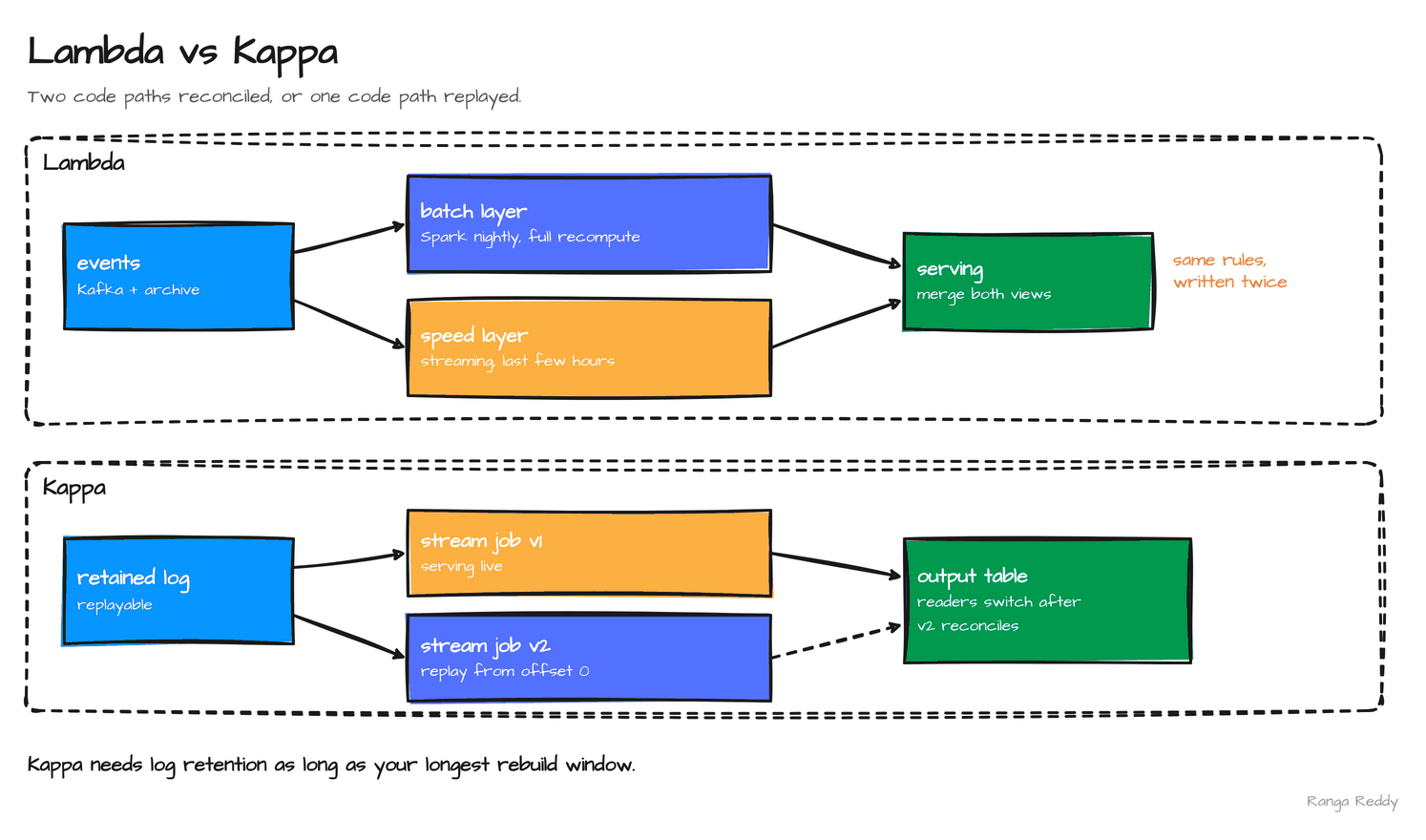
Both patterns address the tension between low-latency updates and the ability to recompute results after code or business rules change.
Lambda runs a batch path for complete recomputation and a speed path for recent changes, and the query layer reconciles both. Separate paths can meet historical and low-latency needs. The cost is business logic written or translated twice, and the two paths can disagree.
Kappa feeds one retained event log into one streaming model, and a replay rebuilds a new output. There is one transformation path and a natural correction story. It requires retained, replayable events, enough capacity to replay, and a safe cutover of the output.
Kappa is not “streaming instead of batch” in every system. A bounded historical replay is still a batch-shaped workload even if it uses the same stream processor and code. If a source log retains only a few days, an arbitrary multi-year rebuild cannot be performed from that log alone. Keep an immutable archive or another reconstruction source when the business requires longer reprocessing windows.
For the sales model, separate arrival time from business event time. A late
sale must join to a customer version valid at order_ts, not to the dimension
row that happened to be current when the stream processed it. A replay must
produce the same fact key and measure or write into a versioned output and
switch readers after reconciliation.
4.2 Decentralized vs. centralized: data mesh vs. data fabric
In plain terms. Data mesh is about people: each business domain owns and publishes its data as a product. Data fabric is about technology: a connected metadata and integration layer that lets you find and access data wherever it lives. A company can use both.
Data mesh is primarily a way to organize analytical ownership around business domains and data products. Data fabric is a broad architectural approach for connecting, governing, and discovering data across systems, often through shared metadata and integration capabilities. They describe different axes and can coexist; neither is a single product or a table schema.
Who owns and serves a domain dataset? In a data mesh, the domain team owns the data product and its quality interface. In a data fabric, shared capabilities connect assets across owners and systems.
What is centralized? A mesh centralizes platform capabilities and federated interoperability rules. A fabric may centralize metadata, integration, governance, and access automation.
What is the main engineering risk? In a mesh, every domain invents incompatible keys, definitions, and SLOs. In a fabric, a central catalog or virtualization layer promises semantics it cannot enforce.
What does it mean for the model? A mesh publishes a documented schema, owner, keys, and change policy per product. A fabric keeps source, logical, and physical metadata discoverable across platforms.
Centralize what creates interoperability: identity domains, schema
compatibility policy, security classifications, and shared dimensions where
their definitions truly match. Decentralize domain-specific meaning and
delivery ownership. If two domains both use a field called customer_id,
that name alone does not prove they identify the same entity.
Data mesh rests on four principles from its original description: domain ownership, data as a product, a self-serve data platform, and federated computational governance. The fourth is the one modeling depends on, because it is where shared keys and conformed dimensions are agreed.
4.3 Metadata and data lineage: the nervous system of a platform
In plain terms. Metadata is data about data: what a column means, who owns the table, when it last loaded. Lineage is the family tree: which sources and jobs produced this table, and which dashboards depend on it.
Metadata describes data and how it is operated. At minimum, distinguish:
- Structural metadata: names, types, nullability, keys, and schema versions.
- Business metadata: definitions, owner, domain, sensitivity, and allowed use.
- Operational metadata: freshness, row counts, quality results, source offsets, and failed runs.
- Lineage: directed relationships from source datasets through jobs and runs to output datasets.
Lineage answers different questions from a catalog. A catalog helps find and understand a dataset; lineage explains where it came from and which consumers may be affected by a change. OpenLineage models jobs, runs, input datasets, output datasets, and extensible facets. A production contract should capture the source version/offset and model version that produced a snapshot, not just the code repository name.
postgres.shop.orders ──> job: cdc_ingest ──> bronze.order_events
                                                   │
                                     job: build_silver
                                                   v
dim_customer ──────────> job: build_fact ──> gold.fact_order_line ──> revenue dashboard

Impact analysis walks right:   change orders.amount -> who breaks?
Root-cause analysis walks left: dashboard is wrong  -> which job, which run?
Metadata is useful only if it is emitted and maintained. Define stable dataset identifiers across environments, include schema and quality facets, and connect run IDs to orchestrator logs. For regulated data, lineage records do not replace access control or retention policy; they make those policies and their effects auditable.
Part 4 interview questions
1. Lambda vs Kappa: which would you pick for a new platform?
Kappa when the source events can be retained (in Kafka with long retention, or archived to object storage) for as long as the longest rebuild window, and one engine can serve both live processing and replay. Lambda when a batch recompute must use data or logic the stream cannot, and you accept maintaining the same rules twice and reconciling them. Most modern lakehouse designs land close to Kappa, with incremental processing on table formats.
2. Data mesh vs data fabric: are they alternatives?
No. Mesh is an organizational model in which domains own data products. Fabric is a technical layer of shared metadata, integration and access automation. A mesh still needs federated governance for shared keys and contracts, and a fabric can provide the discovery and policy tooling for it.
3. What is data lineage, and how would you use it during an incident?
Lineage is the graph from source datasets through jobs and runs to outputs. During an incident, walk upstream from the wrong dashboard to find which job run changed the data and what its inputs were. Before a change, walk downstream to list every consumer that will be affected. Column-level lineage narrows this from tables to fields.
4. Event time vs processing time: why does a model care?
Event time is when the business event happened; processing time is when the pipeline saw it. Type 2 lookups, daily partitions and late-data handling must use event time, or a late order is attributed to the wrong customer version and the wrong day. Keep both: processing time is useful for audits and freshness monitoring.
Part 5: Database Performance & System Scaling
Performance work starts from the physical execution plan and the data shape, not from a list of fashionable techniques. Indexes, partitions, sort order, and sharding solve different problems and carry different write and operating costs.
5.1 Indexing mechanics: B-trees, bitmaps, hash, clustered vs. non-clustered
In plain terms. An index is the index at the back of a book: instead of reading every page to find “Iceberg”, you look it up and jump to page 212. It speeds up reads, but every new page added to the book means updating the index too.
An index is an access structure that helps an engine find rows without examining every data page. Its useful operators depend on the index type and engine.
B-tree
Fits equality, ranges, and ordered scans on sortable values. It adds write amplification and storage, and a low-selectivity predicate may still scan the table.
Hash
Fits equality lookups in engines that support hash indexes. It cannot serve a range or an ordered scan.
Bitmap
Fits low-cardinality analytic predicates in engines that implement bitmap indexes. Update and concurrency behavior are engine-specific, so it is not a general OLTP index.
GIN and inverted indexes
Fit membership tests on arrays, tokens, and other multi-valued structures. Index size and update cost can be high, and the supported operators depend on the engine.
BRIN and min-max summaries
Fit large ranges that are physically correlated with the column, such as append-ordered timestamps. The summaries are coarse, so they return false-positive blocks that still need filtering.
Run it: when PostgreSQL uses an index, and when it does not.
indexes.sql builds 200,000 orders with three indexes: a B-tree on a
selective column, a B-tree on a column where one value covers 90% of rows,
and a BRIN index on an append-ordered timestamp.
-- 200,000 orders: 2,000 customers, one status that covers 90% of rows,
-- and order times that only ever increase.
CREATE TABLE orders_big AS
SELECT g                                          AS order_id,
       'C' || lpad((g % 2000)::text, 4, '0')      AS customer_id,
       CASE WHEN g % 10 = 0 THEN 'CANCELLED'
            ELSE 'COMPLETE' END                   AS status,
       timestamptz '2025-01-01' + g * interval '1 minute' AS ordered_at,
       (g % 500)::numeric(10, 2)                  AS amount
FROM generate_series(1, 200000) AS g;

CREATE INDEX orders_big_customer_btree ON orders_big (customer_id);
CREATE INDEX orders_big_status_btree   ON orders_big (status);
CREATE INDEX orders_big_ordered_brin   ON orders_big USING brin (ordered_at);
ANALYZE orders_big;

-- Selective: about 100 of 200,000 rows.
EXPLAIN (COSTS OFF)
SELECT * FROM orders_big WHERE customer_id = 'C0042';

-- Not selective: 90% of the table. The index exists and is ignored.
EXPLAIN (COSTS OFF)
SELECT * FROM orders_big WHERE status = 'COMPLETE';

-- A one-day range on an append-ordered column: the tiny BRIN index is enough.
EXPLAIN (COSTS OFF)
SELECT count(*) FROM orders_big
WHERE ordered_at >= '2025-02-01' AND ordered_at < '2025-02-02';

SELECT relname, pg_size_pretty(pg_relation_size(oid)) AS size
FROM pg_class
WHERE relname LIKE 'orders_big%'
ORDER BY relname;
EXPLAIN (COSTS OFF) prints the chosen plan without costs or timings:
 Bitmap Heap Scan on orders_big
   Recheck Cond: (customer_id = 'C0042'::text)
   ->  Bitmap Index Scan on orders_big_customer_btree
         Index Cond: (customer_id = 'C0042'::text)

 Seq Scan on orders_big
   Filter: (status = 'COMPLETE'::text)

 Aggregate
   ->  Bitmap Heap Scan on orders_big
         Recheck Cond: ((ordered_at >= '2025-02-01 00:00:00+00'::timestamp with time zone) AND ...)
         ->  Bitmap Index Scan on orders_big_ordered_brin
               Index Cond: ((ordered_at >= '2025-02-01 00:00:00+00'::timestamp with time zone) AND ...)

          relname          |  size
---------------------------+---------
 orders_big                | 14 MB
 orders_big_customer_btree | 1352 kB
 orders_big_ordered_brin   | 24 kB
 orders_big_status_btree   | 1400 kB
The three plans are the lesson. The selective lookup, about 100 of 200,000
rows, uses the B-tree. The status = 'COMPLETE' filter matches 90% of the
table, so the planner reads the table sequentially and ignores an index that
still costs 1,352 kB of storage and slows every insert. The BRIN index answers
a one-day range at 24 kB, about 1/56 of the B-tree’s size, because the
timestamps increase with physical row order. That correlation is the whole
condition: on randomly ordered data a BRIN summary would match nearly every
block range.
“Clustered” and “non-clustered” are not portable physical promises. In SQL
Server, a clustered index defines the row-storage order and a table has one;
non-clustered indexes are separate lookup structures. PostgreSQL’s CLUSTER
rewrites a table in index order as a one-time operation; later inserts and
updates do not continuously preserve that order. State the database when
using these terms.
Open table formats add file- and manifest-level pruning, not a general B-tree over every row. Iceberg can use partition transforms and per-file metrics to skip files; Delta Lake can collect data-skipping statistics and supports Z-ordering. These mechanisms reduce files or row groups read, but do not replace a primary-key index for point lookups in a relational database.
Oracle’s bitmap-index implementation is aimed at read-heavy analytic workloads: updating an indexed value can lock the bitmap entry representing many rows. Do not carry bitmap-index advice from a star-schema warehouse into a high-concurrency transactional workload without checking that engine’s locking and write behavior.
5.2 The query optimization playbook for large databases
In plain terms. Do not guess why a query is slow. Ask the engine for its plan, find the step that reads or moves the most data, and change one thing at a time.
Use the same loop across engines: state the expected access path, inspect the actual plan, measure input and output cardinalities, then change one thing. Validate both semantics and cost after the change.
- Reduce bytes read. Project only required columns, push predicates to the source, and make date/time filters use the model’s declared timezone.
- Check selectivity and statistics. A predicate on a very common value
may make a sequential scan cheaper than random index lookups, as the
statusplan above shows. Refresh statistics after major loads. - Join at the intended grain. Check uniqueness on the dimension side and inspect join estimates versus actual rows. A faster many-to-many join that multiplies measures is still incorrect.
- Look for avoidable exchanges and sorts. Partitioning, bucketing, clustering, and broadcast are workload-dependent; none is automatically beneficial for every query.
- Inspect skew and the long tail. Average task time can hide one hot partition. Compare per-partition rows/bytes and the maximum against the median.
- Tune only after the plan explains the bottleneck. Memory, parallelism, compaction, and file sizing are different controls; increasing one may move cost to shuffle, storage, or planning.
In PostgreSQL, use EXPLAIN (ANALYZE, BUFFERS) carefully: it executes the
statement and can run writes or expensive functions. In Spark, compare the
physical plan with executed SQL metrics; an initial adaptive plan may change
after shuffle statistics arrive. Do not copy one engine’s plan vocabulary
onto another.
5.3 Key considerations for designing scalable database systems
- Choose keys for identity and distribution separately. A sequential surrogate can be an effective dimension key but a hotspot for a distributed write path; a random UUID may spread writes while increasing key size and reducing locality.
- Avoid hot partitions. Tenant, date, or status keys can be extremely skewed. Measure the distribution before choosing a partition key, shard count, or hash strategy.
- Specify uniqueness scope. A key unique inside one shard may not be globally unique. If consumers join across shards, provide a collision-safe global identity or an explicit compound key.
- Account for cross-boundary operations. A join, transaction, or update that spans shards has coordination cost. Data locality helps only when the query’s filters align with the distribution key.
- Make replay and migration part of the design. Preserve source offsets, support rebuilds into a new table, and define how consumers switch to the validated version.
- Set growth and retention policy. Unbounded event retention, indexes, snapshots, and CDC logs all consume storage and can affect recovery time.
Scale is a workload property, not just row count. Include concurrent readers, write rate, skew, latency objectives, and correction/replay windows in the design envelope.
5.4 Partitioning, sharding, and Z-order
In plain terms. Partitioning splits one table into folders, such as one per day, so a query for one day opens one folder. Sharding splits data across separate database servers. Z-ordering sorts data inside files so that rows with similar values on several columns sit close together.
These words are often used interchangeably, but they refer to distinct mechanisms:
Database partitioning splits one logical table into child partitions managed by one database. It prunes ranges or lists, manages lifecycle, and isolates hot data. Too many partitions raise planning and metadata cost, and uniqueness constraints may have to include the partition key.
Sharding splits data across independent database instances or nodes. It scales capacity and isolates failure and load. The costs are cross-shard joins, cross-shard transactions, global uniqueness, and rebalancing.
File partitioning groups files into directories or table partition specs in a lake. It skips files for common predicates and limits the scope of maintenance. High-cardinality partitions create small files and metadata overhead.
Z-ordering is a multi-dimensional locality layout in table formats that support it. It clusters values so file-level statistics can skip more data. It costs a rewrite, its effect drops as more columns are added, and it is implementation-specific.
For Iceberg, partition transforms such as days(order_ts) keep the logical
timestamp column separate from the physical partition values, and partition
specs can evolve. Delta Lake documents ZORDER BY as a mechanism to colocate
related values for data skipping. Do not label an Iceberg sort order as Z-order
or assume every lakehouse reader interprets a vendor-specific layout command.
Partition only when the table size and query pattern justify it. A predicate
on a source date can enable pruning without asking every query writer to
duplicate a hand-maintained event_date column. Verify pruning in the engine
plan and monitor file counts after the write.
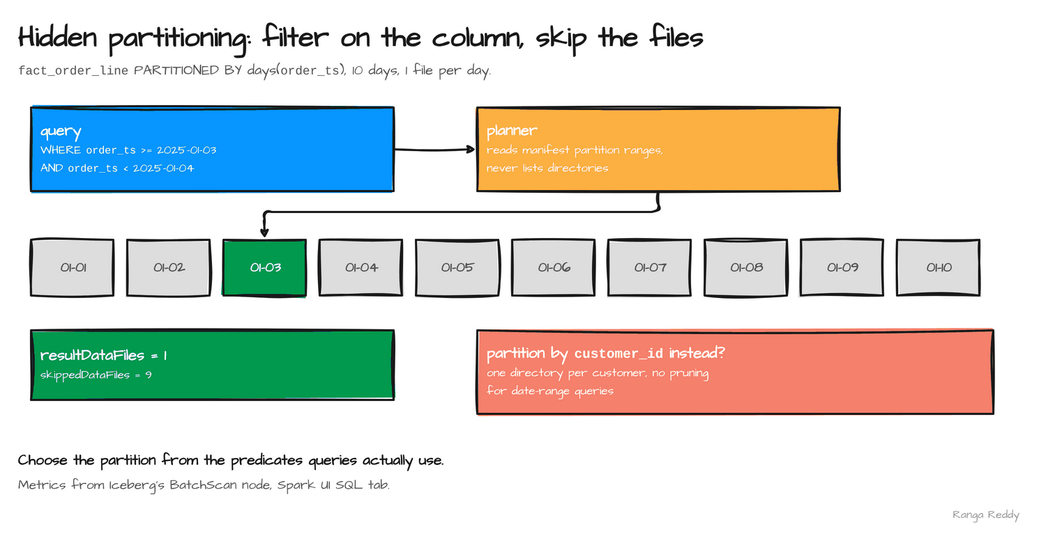
Run it: hidden partitioning and pruning. layout_demo.py writes 10,000
order lines over ten days into an Iceberg table partitioned by
days(order_ts), queries one day by filtering on order_ts itself, and reads
how many data files the scan opened. It then evolves the partition spec to
monthly without rewriting anything:
"""Hidden partitioning on an Iceberg fact table, and what the planner prunes.

The table is partitioned by days(order_ts). Queries filter on order_ts itself;
nobody writes a separate order_date column.
"""
from pyspark.sql import SparkSession

spark = (SparkSession.builder
         .appName("layout-demo")
         .config("spark.sql.extensions",
                 "org.apache.iceberg.spark.extensions.IcebergSparkSessionExtensions")
         .config("spark.serializer", "org.apache.spark.serializer.KryoSerializer")
         .config("spark.sql.catalog.dm", "org.apache.iceberg.spark.SparkCatalog")
         .config("spark.sql.catalog.dm.type", "hadoop")
         .config("spark.sql.catalog.dm.warehouse", "file:///tmp/dm_blog/warehouse")
         .config("spark.sql.session.timeZone", "UTC")
         .getOrCreate())

spark.sql("CREATE NAMESPACE IF NOT EXISTS dm.sales")
spark.sql("DROP TABLE IF EXISTS dm.sales.fact_order_line PURGE")
spark.sql("""
    CREATE TABLE dm.sales.fact_order_line (
        order_id     STRING,
        line_number  INT,
        customer_sk  BIGINT,
        product_sk   BIGINT,
        order_ts     TIMESTAMP,
        quantity     INT,
        net_amount   DECIMAL(12, 2)
    ) USING iceberg
    PARTITIONED BY (days(order_ts))
""")

# 10,000 order lines spread evenly over ten days of January.
spark.sql("""
    INSERT INTO dm.sales.fact_order_line
    SELECT concat('O', id DIV 2)                      AS order_id,
           CAST(id % 2 + 1 AS INT)                    AS line_number,
           id % 500                                   AS customer_sk,
           id % 40                                    AS product_sk,
           TIMESTAMP '2025-01-01' + make_interval(0, 0, 0, 0, 0, 0, id * 86.4) AS order_ts,
           CAST(id % 5 + 1 AS INT)                    AS quantity,
           CAST(id % 100 AS DECIMAL(12, 2))           AS net_amount
    FROM range(10000)
""")

spark.sql("""
    SELECT partition.order_ts_day AS day, record_count, file_count
    FROM dm.sales.fact_order_line.partitions ORDER BY day
""").show()

one_day = """
    SELECT sum(net_amount) FROM dm.sales.fact_order_line
    WHERE order_ts >= TIMESTAMP '2025-01-03' AND order_ts < TIMESTAMP '2025-01-04'
"""
plan = spark.sql("EXPLAIN " + one_day).first()[0]
print([line.strip() for line in plan.splitlines() if "BatchScan" in line][0])


def scan_metrics(df):
    """Iceberg's BatchScan metrics, as the Spark UI SQL tab shows them.

    This reaches into the JVM plan through py4j, which is internal API; it is
    here only to print the numbers without opening the UI.
    """
    df.collect()
    stack = [df._jdf.queryExecution().executedPlan()]
    while stack:
        node = stack.pop()
        if node.nodeName().startswith("BatchScan"):
            m = node.metrics()
            return {k: m.apply(k).value()
                    for k in ("resultDataFiles", "skippedDataFiles")}
        children = node.children().iterator()
        while children.hasNext():
            stack.append(children.next())


spark.conf.set("spark.sql.adaptive.enabled", "false")   # keep the scan node visible
metrics = scan_metrics(spark.sql(one_day))
print("files read vs skipped:", metrics)
assert metrics == {"resultDataFiles": 1, "skippedDataFiles": 9}

assert spark.sql("SELECT count(*) FROM dm.sales.fact_order_line.partitions").first()[0] == 10

# Partition evolution: switch new data to monthly partitions, no rewrite.
spark.sql("ALTER TABLE dm.sales.fact_order_line "
          "REPLACE PARTITION FIELD days(order_ts) WITH months(order_ts)")
spark.sql("""
    INSERT INTO dm.sales.fact_order_line VALUES
    ('O9001', 1, 1, 1, TIMESTAMP '2025-02-14 09:00:00', 1, 10.00)
""")
spark.sql("""
    SELECT spec_id, count(*) AS files FROM dm.sales.fact_order_line.files
    GROUP BY spec_id ORDER BY spec_id
""").show()

print("PASS: 10 day partitions, then a monthly spec added without a rewrite")
spark.stop()
+----------+------------+----------+
|       day|record_count|file_count|
+----------+------------+----------+
|2025-01-01|        1000|         1|
|2025-01-02|        1000|         1|
   ... 7 more days, 1,000 records and 1 file each ...
|2025-01-10|        1000|         1|
+----------+------------+----------+

+- BatchScan dm.sales.fact_order_line[order_ts#63, net_amount#65] dm.sales.fact_order_line (branch=null) [filters=order_ts IS NOT NULL, order_ts >= 1735862400000000, order_ts < 1735948800000000, groupedBy=] RuntimeFilters: []
files read vs skipped: {'resultDataFiles': 1, 'skippedDataFiles': 9}
+-------+-----+
|spec_id|files|
+-------+-----+
|      0|   10|
|      1|    1|
+-------+-----+
PASS: 10 day partitions, then a monthly spec added without a rewrite
The query never mentions a partition column. Iceberg converts the order_ts
range into the days partition values, reads them from the manifests, and
opens 1 of 10 files. The two numbers come from Iceberg’s own scan metrics,
which the Spark UI shows on the BatchScan node. After
REPLACE PARTITION FIELD, the ten old files keep spec_id 0 and the new
February file is written with spec_id 1; no existing file was rewritten,
and queries still filter on order_ts alone.
5.5 ACID vs. BASE and the CAP theorem in modeling
In plain terms. ACID is the bank-transfer promise: money leaves one account and arrives in the other, or neither happens. BASE accepts that copies of the data may briefly disagree, in exchange for staying available. CAP says that when the network between servers breaks, a distributed system must choose between answering with possibly stale data and refusing to answer.
ACID describes transaction properties: atomicity, consistency with declared constraints, isolation, and durability. BASE is a broad descriptive design slogan—basically available, soft state, eventually consistent—not a competing SQL transaction standard. A system can use ACID transactions for an individual write while exposing asynchronously refreshed read models elsewhere.
The two meanings of “consistency” must not be conflated. ACID consistency
means a committed transaction preserves application/database invariants. The
C in CAP concerns whether distributed reads observe a single up-to-date
copy. CAP’s trade-off applies when communication is partitioned: a system
cannot guarantee both linearizable consistency and availability for every
request during that partition. It does not say a normal distributed system
must choose only two properties at all times.
For data models, make the trade visible to consumers. Is a dashboard allowed to read a replica behind the source? Can independent partitions accept writes that may conflict? How will those writes be reconciled, and which business invariants must never be violated? “Eventually consistent” is not a recovery plan; name the lag bound, conflict rule, and reconciliation owner.
5.6 Physical layout: schema versus stored bytes
The star schema says how records relate and what they mean. Physical layout says how bytes are stored and found. Keep those decisions separate so a new partition strategy does not force consumers to rewrite their SQL.
Customer history. The model decides one row per customer version and validity interval. The physical layer decides how to sort or cluster files to help common customer and time lookups.
Sales fact. The model decides one row per order line. The physical layer decides whether to partition by a coarse date transform, once data volume justifies it.
Schema change. The model decides to add sales_channel with a defined
meaning and a default or backfill policy. The physical layer evolves the
table schema, knowing old files may not contain the new field.
Query filters. The model decides that queries use order_date_key and
dimensional keys consistently. The physical layer picks file format,
partition transforms, and clustering from measured queries.
Do not partition a large table by a high-cardinality business key such as
customer_id. That tends to create many small directories and files while
doing little to reduce scans. A coarse event-date transform is often a better
starting point, but the correct choice follows query predicates, file sizes,
and write frequency. Apache Iceberg supports hidden partitioning and partition
evolution, so a logical filter on the source timestamp can remain stable as
the physical partition spec changes. Evolution avoids requiring consumers to
filter on hand-maintained partition columns; it does not remove the need to
measure pruning or file counts.
Schema-on-read formats also need explicit schema discipline. Spark’s Parquet schema merge is disabled by default because merging file schemas has a cost. Do not rely on a random file’s inferred schema to define a production model. Publish an explicit contract, validate incoming schemas, and make compatible evolution deliberate.
5.7 Put model contracts into tests
Every published fact or dimension should have checks that express its contract:
Grain uniqueness. (order_id, line_number) appears at most once in the
transaction fact.
Non-null keys. Every required fact foreign key resolves to a real member or to an explicit unknown member.
Dimension uniqueness. One dimension surrogate key identifies one row.
Type 2 intervals. Versions for one business key never overlap, so an event-time lookup matches at most one version.
Change ordering. A later-arriving source version never overwrites a newer accepted source sequence.
Measure reconciliation. Fact net amount equals gross less discount, under the declared currency and rounding rules.
Batch idempotency. Replaying the same input changes neither row counts nor totals.
Delete semantics. A source delete is retained, invalidated, or stored as a tombstone, by an explicit policy.
The demos in this guide implement most of these as plain assert statements:
grain uniqueness and unknown-member coverage in section 3.5, Type 2
non-overlap in section 3.1, change ordering and replay idempotency in section
3.2. In a production pipeline the same checks run as data-quality tests after
each load and fail the publish step.
Also test volume and operations: rows rejected, unknown-member rates, late arrival age, duplicate source keys, fact-to-source reconciliation, file counts, and model freshness. Alert thresholds should distinguish a newly sparse source from a broken join.
A practical design sequence: identify the business process; write the grain as a sentence; inspect the source’s keys and change semantics; choose transaction, periodic, or accumulating facts; define dimensions and history; specify measures and their aggregation rules; publish the logical contract; then choose the storage layout and test the invariants. Revisit the physical layout when measured access patterns change, not every time a new report is requested.
Part 5 interview questions
1. Why might a database ignore an index on a filtered column?
Because the predicate is not selective. If the filter matches a large share
of the table, following the index means many random page reads, which costs
more than one sequential scan. In the PostgreSQL demo, status = 'COMPLETE'
matches 90% of rows and the planner chooses Seq Scan despite a B-tree on
status. Stale statistics, functions applied to the column, and type
mismatches can also prevent index use.
2. B-tree vs bitmap vs BRIN: when would you use each?
B-tree for selective equality and range lookups, the default for OLTP. Bitmap indexes (in engines such as Oracle) for low-cardinality columns in read-heavy analytic tables, not for concurrent updates. BRIN for very large tables whose physical order follows the column, such as append-only event time, where a tiny summary index skips most blocks. The demo’s BRIN index is 24 kB against 1,352 kB for a B-tree on the same table.
3. Partitioning vs sharding vs bucketing vs Z-ordering.
Partitioning splits one table into parts that queries can skip, inside one system. Sharding spreads data across independent servers to scale capacity, at the cost of cross-shard joins and transactions. Bucketing (in Spark/Hive) hashes rows into a fixed number of files per partition, so joins on the bucket key can avoid a shuffle. Z-ordering (in Delta, for example) sorts rows by several columns at once to improve file-level min/max skipping.
4. How do you choose a partition column for a lakehouse fact table?
From the predicates queries actually use, usually event date. Prefer low to
moderate cardinality so each partition holds well-sized files, and never a
high-cardinality key such as customer_id. In Iceberg, use a transform such
as days(order_ts) so queries filter on the real column, and evolve the spec
later if volume changes. Verify pruning in the scan metrics, as the layout
demo does: 1 file read, 9 skipped.
5. Explain the CAP theorem correctly.
During a network partition, a distributed system must choose between consistency (every read sees the latest write) and availability (every request gets a non-error response). When there is no partition, it can provide both. CAP’s C is not the C of ACID, which means preserving declared invariants inside a transaction.
6. What data quality tests would you put on a fact table?
Grain uniqueness on the declared key, foreign keys that resolve to a real or
unknown member, no NULL in required keys, reconciliation of totals against
the source, idempotency (a replay changes nothing), freshness, and volume
anomaly checks. For a Type 2 dimension, add a no-overlap test and exactly one
current row per business key.
Part 6: Database Lifecycle & Tooling Mechanics
Models move in both directions. Forward engineering turns agreed semantics into schemas, constraints, migrations, and pipelines. Reverse engineering starts from deployed objects and reconstructs their declared structure. Neither direction can infer all the business meaning without people and source documentation.
6.1 Forward engineering vs. reverse engineering
In plain terms. Forward engineering is building the house from the blueprint. Reverse engineering is drawing the blueprint by measuring a house that already exists, and then asking the owners why that one wall is there.
Forward engineering starts from business requirements and a conceptual or logical model. It produces DDL, migration scripts, constraints, transformations, and test contracts. Review whether the design matches what the sources can deliver and what the queries need.
Reverse engineering starts from existing schemas, views, constraints, and observed data. It produces an inventory, an ER diagram, a candidate model, and a dependency graph. Review the grain, hidden application rules, temporal meaning, and undocumented exceptions, because none of them are in the catalog.
Treat deployed schema changes as versioned migrations. A change record should state the contract version, compatibility impact, rollout order, validation, and backfill plan. For a breaking rename, an expand-and-contract rollout can add the new field, dual-write or backfill, migrate consumers, verify the old field is unused, and only then remove it. A rollback script cannot always recover dropped or reinterpreted data, so the recovery plan may be a forward repair rather than a literal inverse migration.
Expand-and-contract rename: cust_no -> customer_id

step 1  expand    add customer_id (nullable)            readers: cust_no
step 2  migrate   backfill + dual-write both columns    readers: either
step 3  switch    move every consumer to customer_id    readers: customer_id
step 4  verify    query logs show no reads of cust_no
step 5  contract  drop cust_no
6.2 How reverse engineering works under the hood
For a relational database, an introspection tool reads the system catalog or standard information schema. It collects columns and types, nullability, defaults, primary/unique/foreign keys, indexes, views, and dependencies. It then maps declared foreign keys to relationship edges and can infer candidate cardinality from uniqueness and nullability constraints.
The distinction between declared and observed is important. A declared foreign key is evidence of an enforced relationship. A frequent join in query logs is only a candidate relationship. A missing foreign key might mean a performance choice, a cross-system relationship, or simply an integrity gap; reverse engineering cannot decide which explanation is correct.
The following read-only PostgreSQL queries list visible columns and declared
foreign-key column mappings. information_schema is SQL-standard and
portable; pg_catalog is PostgreSQL-specific and exposes engine details that
the standard views do not. Run them against the dm_blog database after
normalization.sql, and they recover the 3NF schema and its four foreign keys.
SELECT table_schema,
       table_name,
       ordinal_position,
       column_name,
       data_type,
       is_nullable,
       column_default
FROM information_schema.columns
WHERE table_schema = ANY (current_schemas(false))
ORDER BY table_schema, table_name, ordinal_position;

SELECT source_ns.nspname AS source_schema,
       source_table.relname AS source_table,
       constraint_row.conname AS constraint_name,
       source_column.attname AS source_column,
       target_ns.nspname AS target_schema,
       target_table.relname AS target_table,
       target_column.attname AS target_column,
       source_key.ordinality AS key_position
FROM pg_constraint AS constraint_row
JOIN pg_class AS source_table
  ON source_table.oid = constraint_row.conrelid
JOIN pg_namespace AS source_ns
  ON source_ns.oid = source_table.relnamespace
JOIN pg_class AS target_table
  ON target_table.oid = constraint_row.confrelid
JOIN pg_namespace AS target_ns
  ON target_ns.oid = target_table.relnamespace
JOIN LATERAL unnest(constraint_row.conkey)
  WITH ORDINALITY AS source_key(attnum, ordinality)
  ON true
JOIN LATERAL unnest(constraint_row.confkey)
  WITH ORDINALITY AS target_key(attnum, ordinality)
  ON target_key.ordinality = source_key.ordinality
JOIN pg_attribute AS source_column
  ON source_column.attrelid = source_table.oid
 AND source_column.attnum = source_key.attnum
JOIN pg_attribute AS target_column
  ON target_column.attrelid = target_table.oid
 AND target_column.attnum = target_key.attnum
WHERE constraint_row.contype = 'f'
  AND source_ns.nspname = ANY (current_schemas(false))
ORDER BY source_schema, source_table, constraint_name, key_position;
The second query returns one row per foreign-key column (schema columns trimmed here), which is exactly the edge list of the normalization diagram in section 2.1:
 source_table |       constraint_name        | source_column | target_table | target_column
--------------+------------------------------+---------------+--------------+---------------
 customer     | customer_postal_code_fkey    | postal_code   | postal_area  | postal_code
 order_line   | order_line_order_id_fkey     | order_id      | sales_order  | order_id
 order_line   | order_line_product_id_fkey   | product_id    | product      | product_id
 sales_order  | sales_order_customer_id_fkey | customer_id   | customer     | customer_id
Those queries reveal declared structure, not an ER model ready for publication. Continue by sampling value distributions, checking whether candidate keys are actually unique, examining null rates and orphan rows, and asking the source owners what the fields mean. Then compare the recovered schema to the desired conceptual model: legacy schemas often encode implementation history rather than current business boundaries.
Part 6 interview questions
1. How would you rename a column used by twenty downstream jobs without downtime?
Expand and contract. Add the new column, backfill it, and dual-write both. Migrate consumers one by one while both exist. Confirm from query logs or lineage that nothing reads the old column, then drop it. In Iceberg, a rename is a metadata-only change because columns are tracked by field ID, but your consumers’ SQL still breaks, so the rollout plan is the same.
2. You inherit an undocumented database. How do you model it?
Read the catalog (information_schema, pg_catalog) for tables, types, keys
and declared foreign keys. Profile the data: test candidate keys for
uniqueness, measure null rates, and look for orphan rows. Mine query logs for
frequent joins, which suggest undeclared relationships. Then interview the
owners about grain, time semantics and exceptions, and write a conceptual
model of how the business works, not of how the tables happen to look.
Interview scenario round: design questions
Interviewers for senior roles usually stop asking definitions and hand you a business. These five scenarios cover the patterns above. For each, say the grain sentence first; most of the score is in that sentence.
1. Design the analytical model for a ride-hailing company.
Grain: one row per completed or cancelled trip, in fact_trip. Dimensions:
dim_rider, dim_driver (Type 2 on rating tier and vehicle),
dim_location used twice as pickup and drop-off (role-playing), dim_date
and dim_time. Measures: fare, tip, distance, duration, surge multiplier
(non-additive; store base and surge amounts instead). Driver online hours are
a different process, so they get their own fact, such as
fact_driver_session or a daily periodic snapshot of driver activity.
Partition fact_trip by days(pickup_ts).
2. Model subscription revenue so that monthly recurring revenue (MRR) is easy to report.
Keep fact_subscription_event as a transaction fact, with one row per
start, upgrade, downgrade or cancel. Add fact_subscription_monthly, a
periodic snapshot with one row per subscription per month holding MRR and
status. MRR is semi-additive: sum it across customers within a month, never
across months. Churn and expansion come from comparing consecutive snapshots.
The customer dimension is Type 2 on plan and segment, so cohort reports use
the plan at the time.
3. Track e-commerce orders from placement to delivery and report average delivery time.
An accumulating snapshot: one row per order with ordered_ts, paid_ts,
shipped_ts and delivered_ts, and the lag measures between them, updated
in place as each milestone arrives (a MERGE keyed on order_id). Use
role-playing date keys for each milestone. Keep the line-level transaction
fact for revenue; the two facts answer different questions and share
conformed dimensions.
4. Build a CDC pipeline from PostgreSQL to a lakehouse with a Type 2 customer dimension.
Debezium reads the WAL and publishes snapshot plus change events to Kafka.
Land them unchanged in a bronze Iceberg table with key, op, LSN and payload.
In silver, deduplicate on (key, lsn) and keep the latest event per key per
batch. Apply a current-state MERGE guarded by lsn > target_lsn, with
tombstones for deletes. Build dim_customer with the two-row staging MERGE
from section 3.1, using the source’s business effective time for
valid_from. Test replay idempotency, Type 2 non-overlap, and key coverage
before publishing gold.
5. The revenue dashboard shows double yesterday's number. How do you debug it?
Check grain before tuning anything. First, run uniqueness on the fact key; if there are duplicates, check whether a retry appended a batch twice (non-idempotent load). Second, check each dimension join: count rows before and after; a Type 2 join on the business key alone, or a bridge without weights, multiplies rows. Third, compare against the source total for the same event-time window. Then walk the lineage upstream to the job run that changed. The demos in this guide reproduce two of these causes exactly.
Summary and key takeaways
Modeling is the work of making data interpretable without making every consumer rediscover how it was produced. Start with a row-level business contract, preserve the identity and relevant history of each dimension, and keep facts at a consistent grain. Then prove the contract with data tests.
The durable distinctions are simple:
- The business key identifies an entity; the surrogate key identifies a warehouse row or historical version.
- Event time says when a business event occurred; processing time says when the platform handled it.
- A logical model defines grain and relationships; a physical table layout defines where bytes land and which files a query can skip.
- Atomic commits protect table metadata; idempotent transformations protect business outcomes when inputs are replayed.
When a total changes unexpectedly, verify grain and join cardinality before tuning Spark. When history looks wrong, verify validity intervals and event time before changing a table format. Those checks find modeling errors closer to their cause than another layer of SQL can.
For interview preparation, practise saying each idea at three depths: the one-sentence “in plain terms” version, the mechanism with its trade-off, and a concrete number from one of the demos. That last step is what separates a memorized answer from one that has been run.
References
- Declaring the grain and fact tables for grain discipline and transaction, periodic snapshot, and accumulating snapshot patterns
- Design Tip #152: SCD Types 0, 4, 5, 6 and 7 and Slowly Changing Dimensions for Type 0–6 behavior and historical change policies
- Understand star schema for fact and dimension responsibilities, surrogate keys, and Type 1/2 examples
- UC Berkeley CS 186 database design notes for ER constraints, functional dependencies, BCNF, and lossless decomposition
- Oracle SQL Tuning Guide: optimizer access paths for B-tree, bitmap, table-cluster, and optimizer access-path behavior in Oracle
- DataVault4dbt staging for a practical Data Vault staging implementation
- Data lakehouse overview for the broad platform comparison
- Medallion architecture for bronze, silver, and gold layer responsibilities and operational guidance
- dbt snapshots for a practical implementation of Type 2 history over mutable source tables
- Debezium PostgreSQL connector for snapshot-plus-log CDC, keys, operation envelopes, source positions, and delete/tombstone events
- Spark 3.5.9 CREATE TABLE USING and Parquet data source behavior for Spark table DDL, partition discovery, and Parquet schema merging
- Iceberg 1.11.0 schema and partition evolution and partitioning for separating logical columns from physical layout
- Iceberg 1.11.0 Spark writes for
MERGE INTOsemantics, and Spark DDL forREPLACE PARTITION FIELD - Delta Lake Z-ordering and data skipping for a format-specific example of file-level locality
- PostgreSQL index types, BRIN indexes,
CLUSTER, partitioning, and information schema for the engine-specific indexing, storage, and reverse-engineering examples - Spark SQL performance tuning for query-plan and adaptive-execution tuning concepts
- Data Mesh Principles and Logical Architecture, IBM data mesh, and IBM data fabric for the distinct ownership and integration concerns
- Questioning the Lambda Architecture for the dual-path cost and replay-centered alternative
- CAP Twelve Years Later for the partition-time scope of CAP and its distinction from ACID consistency
- OpenLineage facets for run, job, dataset, and extensible lineage metadata
- Run every demo on this blog locally for the public Spark and lakehouse playground setup
Trademarks
Apache Spark, Apache Iceberg, Apache Parquet and Apache are either registered trademarks or trademarks of The Apache Software Foundation in the United States and other countries.
Found this useful?
These posts and tools are free. If one saved you an afternoon, you can buy me a coffee.